11.1E: Exercises

Exercises

1. The sounds we hear are made up of mechanical waves. The note ‘A’ above the note ‘middle C’ is a sound wave with ordinary frequency \(f=440 \text { Hertz }=440 \frac{\text { cycles }}{\text { second }}\). Find a sinusoid which models this note, assuming that the amplitude is 1 and the phase shift is 0.
2. The voltage \(V\) in an alternating current source has amplitude \(220 \sqrt{2}\) and ordinary frequency \(f=60 \text { Hertz }\). Find a sinusoid which models this voltage. Assume that the phase is 0.
3. The London Eye is a popular tourist attraction in London, England and is one of the largest Ferris Wheels in the world. It has a diameter of 135 meters and makes one revolution (counterclockwise) every 30 minutes. It is constructed so that the lowest part of the Eye reaches ground level, enabling passengers to simply walk on to, and off of, the ride. Find a sinusoid which models the height \(h\) of the passenger above the ground in meters \(t\) minutes after they board the Eye at ground level.
4. On page 732 in Section 10.2, we found the \(x\)-coordinate of counter-clockwise motion on a circle of radius \(r\) with angular frequency \(\omega\) to be \(x=r \cos (\omega t)\), where \(t = 0\) corresponds to the point \((r, 0)\). Suppose we are in the situation of Exercise 3 above. Find a sinusoid which models the horizontal displacement \(x\) of the passenger from the center of the Eye in meters \(t\) minutes after they board the Eye. Here we take \(x(t)>0\) to mean the passenger is to the right of the center, while \(x(t)<0\) means the passenger is to the left of the center.
5. In Exercise 52 in Section 10.1, we introduced the yo-yo trick ‘Around the World’ in which a yo-yo is thrown so it sweeps out a vertical circle. As in that exercise, suppose the yo-yo string is 28 inches and it completes one revolution in 3 seconds. If the closest the yo-yo ever gets to the ground is 2 inches, find a sinusoid which models the height \(h\) of the yo-yo above the ground in inches \(t\) seconds after it leaves its lowest point.
6. Suppose an object weighing 10 pounds is suspended from the ceiling by a spring which stretches 2 feet to its equilibrium position when the object is attached.
   1. Find the spring constant \(k\) in \(\frac{\text{lbs} .}{\text{ft} .}\) and the mass of the object in slugs.
   2. Find the equation of motion of the object if it is released from 1 foot below the equilibrium position from rest. When is the first time the object passes through the equilibrium position? In which direction is it heading?
   3. Find the equation of motion of the object if it is released from 6 inches above the equilibrium position with a downward velocity of 2 feet per second. Find when the object passes through the equilibrium position heading downwards for the third time.
7. 

   \[T=2 \pi \sqrt{\frac{l}{g}}\nonumber\]

   where \(l\) is the length of the pendulum and \(g\) is the acceleration due to gravity.

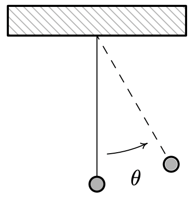
   1. Find a sinusoid which gives the angular displacement \(\theta\) as a function of time, \(t\). Arrange things so \(\theta(0)=\theta_{0}\).
   2. In Exercise 40 of section 5.3, you found the length of the pendulum needed in Jeff’s antique Seth-Thomas clock to ensure the period of the pendulum is \(\frac{1}{2}\) of a second. Assuming the initial displacement of the pendulum is \(15^{\circ}\), find a sinusoid which models the displacement of the pendulum \(\theta\) as a function of time, \(t\), in seconds.
8. The table below lists the average temperature of Lake Erie as measured in Cleveland, Ohio on the first of the month for each month during the years 1971 – 2000.¹⁹ For example, \(t = 3\) represents the average of the temperatures recorded for Lake Erie on every March 1 for the years 1971 through 2000.

   \[\begin{array}{|l|r|r|r|r|r|r|r|r|r|r|r|r|} \hline \begin{array}{l} \text { Month } \\ \text { Number, } t \end{array} & 1 & 2 & 3 & 4 & 5 & 6 & 7 & 8 & 9 & 10 & 11 & 12 \\
   \hline \begin{array}{l} \text { Temperature } \\ \left({ }^{\circ} \mathrm{F}\right), T \end{array} & 36 & 33 & 34 & 38 & 47 & 57 & 67 & 74 & 73 & 67 & 56 & 46 \\ \hline
   \end{array}\nonumber\]

   1. Fit a sinusoid to these data.
   2. Using a graphing utility, graph your model along with the data set to judge the reasonableness of the fit.
   3. Use the model you found in part 8a to predict the average temperature recorded for Lake Erie on April 15^th and September 15^th during the years 1971–2000.²⁰
   4. Compare your results to those obtained using a graphing utility.
9. The fraction of the moon illuminated at midnight Eastern Standard Time on the \(t^{\text {th }}\) day of June, 2009 is given in the table below.²¹
   1. Fit a sinusoid to these data.
   2. Using a graphing utility, graph your model along with the data set to judge the reasonableness of the fit.
   3. Use the model you found in part 9a to predict the fraction of the moon illuminated on June 1, 2009.
   4. Compare your results to those obtained using a graphing utility.

Answers

1. \(S(t)=\sin (880 \pi t)\)
2. \(V(t)=220 \sqrt{2} \sin (120 \pi t)\)
3. \(h(t)=28 \sin \left(\frac{2 \pi}{3} t-\frac{\pi}{2}\right)+30\)
4. \(x(t)=67.5 \cos \left(\frac{\pi}{15} t-\frac{\pi}{2}\right)=67.5 \sin \left(\frac{\pi}{15} t\right)\)
5. \(h(t)=28 \sin \left(\frac{2 \pi}{3} t-\frac{\pi}{2}\right)+30\)
6. 1. \(k=5 \frac{\text { lbs. }}{\text { ft. }} \text { and } m=\frac{5}{16} \text { slugs }\)
   2. \(x(t)=\sin \left(4 t+\frac{\pi}{2}\right)\). The object first passes through the equilibrium point when \(t=\frac{\pi}{8} \approx 0.39\) 0.39 seconds after the motion starts. At this time, the object is heading upwards.
   3. \(x(t)=\frac{\sqrt{2}}{2} \sin \left(4 t+\frac{7 \pi}{4}\right)\). The object passes through the equilibrium point heading downwards for the third time when \(t=\frac{17 \pi}{16} \approx 3.34\) seconds.
7. 1. \(\theta(t)=\theta_{0} \sin \left(\sqrt{\frac{g}{l}} t+\frac{\pi}{2}\right)\)
   2. \(\theta(t)=\frac{\pi}{12} \sin \left(4 \pi t+\frac{\pi}{2}\right)\)
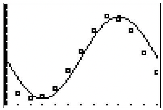
8. 1. \(T(t)=20.5 \sin \left(\frac{\pi}{6} t-\pi\right)+53.5\)
   2. Our function and the data set are graphed below. The sinusoid seems to be shifted to the right of our data.

      

   3. The average temperature April \(15^{\text {th }}\) is approximately \(T(4.5) \approx 39.00^{\circ} \mathrm{F}\) and the average temperature on September \(15^{\text {th }}\) is approximately \(T(9.5) \approx 73.38^{\circ} \mathrm{F}\).
   4. Using a graphing calculator, we get the following

      

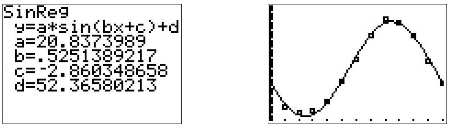
      This model predicts the average temperature for April \(15^{\mathrm{th}}\) to be approximately \(42.43^{\circ} \mathrm{F}\) and the average temperature on September \(15^{\text {th }}\) to be approximately \(70.05^{\circ} \mathrm{F}\). This model appears to be more accurate.

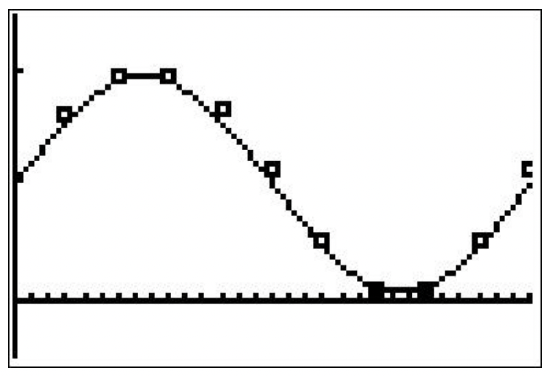
9. 1. Based on the shape of the data, we either choose \(A<0\) or we find the second value of \(t\) which closely approximates the ‘baseline’ value, \(F=0.505\). We choose the latter to obtain \(F(t)=0.475 \sin \left(\frac{\pi}{15} t-2 \pi\right)+0.505=0.475 \sin \left(\frac{\pi}{15} t\right)+0.505\).
   2. Our function and the data set are graphed below. It’s a pretty good fit.

      

   3. The fraction of the moon illuminated on June 1st, 2009 is approximately \(F(1) \approx 0.60\)
   4. Using a graphing calculator, we get the following.

      

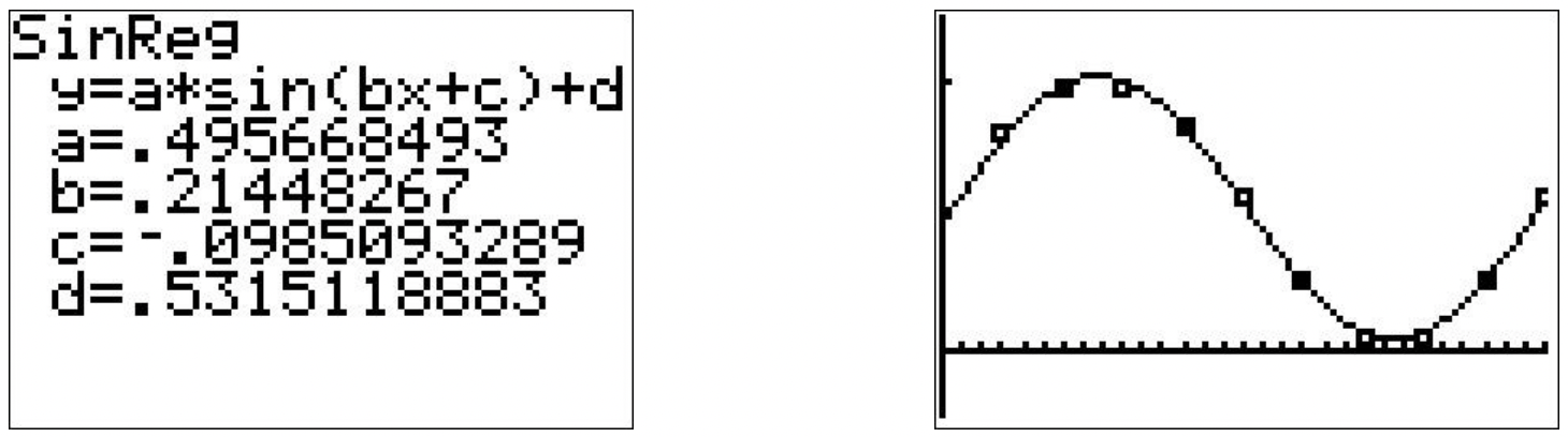
      This model predicts that the fraction of the moon illuminated on June 1st, 2009 is approximately 0.59. This appears to be a better fit to the data than our first model.