5.4: Sinusoidal Models

Suggested Prerequisite Topics

This section is designed assuming you understand the following topics from Algebra.

• Building linear and quadratic models from applications and data.

Learning Objectives

• Build a sinusoidal model from an application.
• Build a sinusoidal model from data.

Rewriting the Coordinate Definition

We begin this section with a brief interlude. Recall the coordinate definition of the trigonometric functions, which is presented below for our discussion.

Definition: Trigonometric Functions (Coordinate Definition)

Let \( \theta \) be an angle in standard position with the point \( P\left( x,y \right) \) on the terminal side of \( \theta \), where \( P \) is not the origin. Define \( r = \sqrt{x^2 + y^2} \). The trigonometric functions of the angle \( \theta \) are defined as follows:\[ \begin{array}{|cccc|cccc|}
\hline
\text{Function} & \text{Function} & & & \text{Function} & \text{Function} & & \\
\text{Name} & \text{Notation} & & \text{Definition} & \text{Name} & \text{Notation} & & \text{Definition} \\
\hline
\text{The sine of }\theta & \sin\left( \theta \right) & = & \dfrac{y}{r} & \text{The cosecant of }\theta & \csc\left( \theta \right) & = & \dfrac{r}{y} \\
\text{The cosine of }\theta & \cos\left( \theta \right) & = & \dfrac{x}{r} & \text{The secant of }\theta & \sec\left( \theta \right) & = & \dfrac{r}{x} \\
\text{The tangent of }\theta & \tan\left( \theta \right) & = & \dfrac{y}{x} & \text{The cotangent of }\theta & \cot\left( \theta \right) & = & \dfrac{x}{y} \\
\hline \end{array} \nonumber \]

If we hold \( r \) to be constant and plot all points a distance of \( r \) units from the origin, then we will have graphed a circle of radius \( r \) centered at the origin. By the coordinate definition of the trigonometric functions, if the point \( \left( x,y \right) \) is on this circle and is on the terminal side of \( \theta \), then\[ \cos\left( \theta \right) = \dfrac{x}{r} \quad \text{and} \quad \sin\left( \theta \right) = \dfrac{y}{r}. \nonumber \]We have reached a point in this text where writing these formulas in an alternate form is more useful. Solving the formulas for \( x \) and \( y \), respectively, we get the following:\[ x = r \cos\left( \theta \right) \quad \text{and} \quad y = r \sin\left( \theta \right). \label{polarform} \]The formulas in \ref{polarform} apply to any point on the terminal side of \( \theta \) on a circle of radius \( r \). Understanding these formulas is essential for our success moving forward in Trigonometry.

Sinusoidal Models

Now that we have a solid understanding of the graphs for the fundamental trigonometric functions, it's time we focused on their applications. In the same way exponential functions can be used to model a wide variety of phenomena in nature, the cosine and sine functions can be used to model their fair share of natural behaviors. In particular, sinusoidal waves are common in physics, engineering, computer science, signal processing, and many other fields. For consistency, we will focus on building applications using the sine function.¹ Moreover, we switch to the independent variable \(t\) (instead of \( x \) or \( \theta \)) since the applications in this section are time-dependent.

Before diving into the applications, let's summarize some important facts and definitions about the sine function. Let\[ f(t) = A \, \sin\left( Bt + C \right) + D. \label{sinefnc} \]From the material so far in this chapter, we know that \( |A| \) is the amplitude, the period is \( \frac{2\pi}{B} \), the phase shift is \( -\frac{C}{B} \), and the vertical shift (or midline) is \( D \).

Along with knowing these formulas, it is helpful to remember what these quantities mean in context. As we discuss these contextual meanings, we will inevitably introduce more definitions (mostly from physics) that we will occasionally be using throughout the remainder of this text.

• The amplitude measures the sine wave's maximum displacement (change in position) from its midline. Therefore, if the midline of a sinusoidal function is \( y = 120 \) and the amplitude is \( 30 \), the maximum displacement of the sinusoidal wave is \( 30 \).
• The period is the length of time it takes to complete one cycle of the sinusoid. For a slightly oversimplified example, the signal your antenna is receiving from a broadcasting radio station is a sinusoidal wave. If this wave takes \( 1.0152 \times 10^{-8} \) seconds to complete a single cycle, then its period is \( 1.0152 \times 10^{-8} \).
  • A more physically interesting, and important, interpretation related to the period is the ordinary frequency of the sinusoid (often just called the frequency). This is the number of cycles the sinusoid goes through in a given unit of time (generally, per second). Since the period is in seconds per cycle and frequency is cycles per second, it should make sense that period and frequency are reciprocals. That is, if \( f \) is the frequency of a sinusoid and \( T \) is its period,\[ f = \dfrac{1}{T} \quad \text{and} \quad T = \dfrac{1}{f}.\nonumber \]Thus, the frequency of the radio station mentioned above is\[ f = \dfrac{1}{T} = \dfrac{1}{1.0152 \times 10^{-8}} \approx 98,502,758 \, \text{cycles per second}. \nonumber \]The unit for "cycles per second" is called the Hertz (Hz). Therefore, the radio station is operating at roughly \( 98.5 \) million Hertz, or \( 98.5 \) MHz (megahertz).²
  • Another frequency gets referenced occasionally (albeit less frequently than the ordinary frequency). This is the angular frequency. In terms of Equation \ref{sinefnc}, the angular frequency is defined as the value of \( B \). This tells how many cycles are completed over an interval of length \(2 \pi\).
• The phase shift represents how much of a "head start" the sinusoid has over the unshifted sine function.
  • The phase angle (also called the phase), which was only mentioned in a footnote in the previous section, is the value of \( C \). It is the angle corresponding to \(t = 0\).

All of this information is summarized below.

Summary: Sine Curve Properties

• The amplitude is \( |A| \)
• The angular frequency is \( B \) and the ordinary frequency is \(f=\frac{B}{2 \pi}\)
• The period is \(T = \frac{2 \pi}{B} = \frac{1}{f}\)
• The phase angle is \( C \) and the phase shift is \(-\frac{C}{B}\)
• The vertical shift or midline is D

From this point forward, when dealing with applications, we will use the terms angular frequency, frequency, and phase when possible. Therefore, it's best to make a note of these definitions so you don't forget them.

Our first foray into sinusoidal motion puts these definitions and the equations in \ref{polarform} to good use.

Example \( \PageIndex{1} \)

The Giant Wheel at Cedar Point is a circle with a diameter of 128 feet, which sits on an 8-foot-tall platform, making its overall height 136 feet. It completes two revolutions in 2 minutes and 7 seconds. Assuming that the riders are at the edge of the circle, find a sinusoid that describes the height of the passengers above the ground \(t\) seconds after they pass the point on the wheel closest to the ground.

Solution

As is most often the case, we begin by sketching the situation below. We will assume a counter-clockwise rotation.³

We were told the diameter of the circle is 128 feet. Therefore, its radius is 64 feet. For simplicity, and to introduce a coordinate system to the situation, let's graph this circle centered at the origin. We will raise it up eventually, but this initial sketch can be very helpful.

Our eventual goal is to find the height of a rider, which is related to the \( y \)-coordinates of this circle. However, we know from \ref{polarform} that\[ y = r \sin\left( \theta \right) = 64 \sin\left( \theta \right). \nonumber \]One thing you must get used to is that our sinusoidal models are functions of time - not angles. Therefore, we will trade \( \theta \) out for \( B t + C \) - this is the most general argument of the sine function and something we have been working with recently. Hence, the height of a rider on the Great Wheel will be related to the function\[64 \sin\left( \theta \right) = 64 \sin \left( Bt + C \right).\nonumber\]Since the Great Wheel is not partially underground, we need to lift this function up. Specifically, we need to shift the center of our circle so that the bottom of the Great Wheel is \( 8 \) feet above the ground (which is the \( x \)-axis in our figure above). Thus, we need to move this circle up \( 64 \) feet plus an additional \( 8 \) feet, for a total of \( 72 \) feet.

Therefore, we are considering a sinusoidal model of the form\[ h(t) = 64 \sin\left( B t + C\right) + 72. \nonumber \]There are only two things left to consider - the angular frequency and the phase angle of the sinusoidal model.⁴

The angular frequency is \( B \), which is know is related to the period, \( T \), by the formula\[ T = \dfrac{2\pi}{B} \nonumber \]\[\implies B = \dfrac{2 \pi}{T}. \label{ex1formula} \]The period is the time it takes for the sinusoidal function to complete one cycle. For this application, the period is the time it takes the Giant Wheel to perform one full revolution. We are told the Giant Wheel goes through two full revolutions in 2 minutes and 7 seconds. Therefore, it takes 127 seconds to go through two revolutions and half that to go through one. Hence, the period is\[ \text{Period} = T = \dfrac{\text{time}}{\text{one revolution}} = \dfrac{127}{2} \text{ seconds per revolution}. \nonumber \]Substituting this into \ref{ex1formula}, we get\[ B = \dfrac{2 \pi}{T} = \dfrac{2 \pi}{127/2} = \dfrac{4 \pi}{127}. \nonumber \]The sinusoidal model is really taking shape now.\[ h(t) = 64 \sin{\left( \frac{4 \pi}{127} t + C \right)} + 72. \nonumber \]The height of a rider at \( t = 0 \) is \( 8 \). Therefore, letting \( t = 0 \) and \( h = 8 \), we get\[ 8 = 64 \sin\left( C \right) + 72 \implies -1 = \sin\left( C \right) \implies C = \dfrac{3\pi}{2}. \nonumber \]With this, we have found the equation of motion for the rider,\[ h(t) = 64 \sin{\left( \frac{4 \pi}{127} t + \frac{3\pi}{2} \right)} + 72. \nonumber \]We can check the reasonableness of our answer by graphing \(y = h(t)\) over the interval \(\left[0, \frac{127}{2}\right]\).

A few remarks about Example \( \PageIndex{1} \) are in order. First, note that the amplitude of 64 in our answer corresponds to the radius of the Giant Wheel. This means that passengers on the Giant Wheel never stray more than 64 feet vertically from the center of the Wheel, which makes sense. Another way to say this (using our new definitions) is that the maximum displacement of a rider on the Great Wheel is 64 feet.

The second thing to note is our process of finding the value of the phase angle. Trigonometry is a fun topic because there are usually several ways to do something, and not one is better than another. In fact, if I were investigating this problem and were not concerned about instructing you on new language, I would have found the value of \( C \) using a different approach. To figure out the phase angle, we could have sketched the path of a rider on the Great Wheel from the time they enter \(\left( t = 0 \right)\).

Notice that this sketch looks more like a reflected cosine than a sine; however, we made our choice to work with sine, and, darn it, we are going to stick with it. The actual sine function starts one-fourth of the way through this cycle. That is, at time \( \frac{1}{4} \left( \frac{127}{2} \right) = \frac{127}{8} \). Hence, the sinusoidal model has a phase shift of \( \frac{127}{8} \). Using the relation \( \text{Phase Shift} = -\frac{C}{B} \), we get\[ \begin{array}{crcl}
& \text{Phase Shift} & = & -\dfrac{C}{B} \\
\implies & \dfrac{127}{8} & = & -\dfrac{C}{4 \pi/127} \\
\implies & \dfrac{127}{8} & = & -\dfrac{127 C}{4 \pi} \\
\implies & -\dfrac{4 \pi}{8} & = & C \\
\implies & -\dfrac{\pi}{2} & = & C \\
\end{array} \nonumber \]Thus, our sinusoidal model is\[ h(t) = 64 \sin{\left( \frac{4 \pi}{127} t - \frac{\pi}{2} \right)} + 72. \nonumber \]Now, you might say, "Hey, that's not what we got in Example \( \PageIndex{ 1 } \)!" I beg to differ. Remember, the value of \( \sin\left( \theta \right) \) is the same as the value of \( \sin\left( \theta - 2\pi \right) \). If you subtract \( 2\pi \) from the argument in the answer to Example \( \PageIndex{ 1 } \), you would get \( h(t) = 64 \sin{\left( \frac{4 \pi}{127} t - \frac{\pi}{2} \right)} + 72 \).

The third and final thing to mention is the phase shift of our answer, which is \(\frac{127}{8}=15.875\). This represents the "time delay" (in seconds) we introduce by starting the motion at the point \(P\) as opposed to the point \(Q\). Said differently, passengers who "start" at \(P\) take 15.875 seconds to "catch up" to the point \(Q\).

Checkpoint \(\PageIndex{1}\)

Outside temperature over a day can be modeled as a sinusoidal function. Suppose you know the high temperature for the day is 78 degrees and the low temperature of 42 degrees occurs at 6 AM. Assuming \(t\) is the number of hours since midnight, find an equation for the temperature, \( T \), in terms of \(t\).

Answer

\( T(t) = 60 + 18 \sin\left( \frac{\pi}{12}t - \pi \right) \)

Our next example shows how to deal with data that is sinusoidal in nature.

Example \( \PageIndex{2} \)

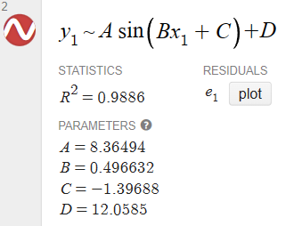
According to the U.S. Naval Observatory website, the number of hours, \(H\), of daylight that Fairbanks, Alaska received on the 21^st day of the \(n\)th month of 2009 is given below. Here, \(t = 1\) represents January 21, 2009, \(t = 2\) represents February 21, 2009, and so on.

\[ \begin{array}{|l|r|r|r|r|r|r|r|r|r|r|r|r|} \hline \begin{array}{l} \text { Month } \\ \text { Number } \end{array} & 1 & 2 & 3 & 4 & 5 & 6 & 7 & 8 & 9 & 10 & 11 & 12 \\ \hline \begin{array}{l} \text { Hours of } \\ \text { Daylight } \end{array} & 5.8 & 9.3 & 12.4 & 15.9 & 19.4 & 21.8 & 19.4 & 15.6 & 12.4 & 9.1 & 5.6 & 3.3 \\ \hline \end{array}\nonumber\]

1. Find a sinusoid that models these data and use graphing technology to graph your answer along with the data.
2. Compare your answer to part (a) to one obtained using the regression feature of your graphing technology.

Solutions

1. We plot the data below (using Desmos' table feature) to get a feel for it.

   

   The data certainly appear sinusoidal,⁵ but when it comes down to it, manually fitting a sinusoid to data is not an exact science. We do our best to find the constants \(A, B, C\) and \(D\) so that the function\[H(t)=A \sin (B t+C)+D\nonumber \]closely matches the data. We first go after the vertical shift \(D\) whose value determines the midline. In a typical sinusoid, the value of \(D\) is the average of the maximum and minimum values. So here we take\[D=\dfrac{3.3+21.8}{2}=12.55.\nonumber\]Next is the amplitude, \(|A|\), which is the displacement from the midline to the maximum (and minimum) values. We find\[|A|=|21.8-12.55|=9.25.\nonumber\]As long as we know we are going to choose our sine function to be positive, we have\[H(t)=9.25 \sin (B t+C)+12.55.\nonumber\]Next, we go after the angular frequency, \(B\). Since the data collected is over the span of a year (12 months), we take the period to be \(T=12\) months.⁶ This means\[B=\frac{2 \pi}{T}=\frac{2 \pi}{12}=\frac{\pi}{6}.\nonumber\]The last quantity to find is the phase, \(C\). It is easier in this case to find the phase shift, \(-\frac{C}{B}\). Since we picked \(A \gt 0\), the phase shift corresponds to the first value of \(t\) with \(H(t) = 12.55\) (the midline value). Here, we choose \(t = 3\), since the output of 12.4 is closer to 12.55 than the next value, 15.9, which corresponds to \(t = 4\). Hence, \(-\frac{C}{B}=3\), so \(C=-3 B=-3\left(\frac{\pi}{6}\right)=-\frac{\pi}{2}\). Thus, we have\[H(t)=9.25 \sin \left(\frac{\pi}{6} t-\frac{\pi}{2}\right)+12.55.\nonumber\]Below is a graph of our data with the curve \(y = H(t)\).

   

2. Using the following command in Desmos, we get

   

   While both models seem to fit the data reasonably, Desmos' model is the better fit.

Checkpoint \( \PageIndex{ 2 } \)

The table shows the number of hours of daylight in Glasgow, Scotland on the first of each month.

Month	Jan	Feb	Mar	Apr	May	Jun	Jul	Aug	Sep	Oct	Nov	Dec
Daylight Hours	7.1	8.7	10.7	13.1	15.3	17.2	17.5	16.7	13.8	11.5	9.2	7.5

1. Sketch a sinusoidal graph of daylight hours as a function of time, with \(t=1\) in January.
2. Estimate the period, amplitude, and midline of the graph.

Answers

1. Plot the data points and fit a sinusoidal curve by eye, as shown below.

   

2. The period of the graph is 12 months. The midline is approximately \(y = 12.25\), and the amplitude is approximately 5.25.

---

Footnotes

¹ If you want to build models based on the cosine function, you are welcome to use the Cofunction Identities we encountered previously to transform our sine models into cosine models.

² If you live in Sacramento, California, this is the frequency for the radio station 98.5 FM KRXQ.

³ Otherwise, we could observe the motion of the wheel from the other side.

⁴ I warned you that we were going to be using that new language. Remember, "angular frequency" is the value of \( B \) and the "phase angle" is the value of \( C \).

⁵ Okay, it appears to be a "V" shape. Just humor me for a moment.

⁶ Even though the data collected lies in the interval \([1, 12]\), which has a length of 11, we need to think of the data point at \(t = 1\) as a representative sample of the amount of daylight for every day in January. That is, it represents \(H(t)\) over the interval \([0, 1]\). Similarly, \(t=2\) is a sample of \(H(t)\) over \([1, 2]\), and so forth.

---

Skills Refresher

Review the following skills you will need for this section.

Skills Refresher

Need some

---

Homework

Vocabulary Check

1. Change in position is also known as ___.

2. The period of a function measures the number of ___ per ___.

3. The ordinary frequency (or, simply, frequency) of a sinusoid measures the number of ___ per ___.

4. The unit for frequency is the ___.

5. In the function\[ f(t) = A\,\sin\left( Bt + C \right) + D, \nonumber \]\( B \) is called the ___, \( C \) is called the ___, and \( -\frac{C}{B} \) is called the ___.

Concept Check

True or False? For Problems 6 - 10, determine if the statement is true or false. If true, cite the definition or theorem stated in the text supporting your claim. If false, explain why it is false and, if possible, correct the statement.

The following questions concern the sinusoidal function\[ f(t) = A \, \sin\left( Bt + C \right) + D. \nonumber \]

6. \( B \) is the period

7. \( C \) is the phase shift

8. \( y = D \) is the midline

9. \( -\frac{C}{B} \) is the phase shift

10. If \( T \) is the period of the sinusoid and \( f \) is the frequency, \( f = \frac{1}{T} \).

Basic Skills

In Problems 11 - 14,
(a) Estimate the amplitude, period, and midline of a sinusoidal function that fits the data.
(b)Write a formula for the function.

11.  

    \(t\)	0	0.25	0.5	0.75	1	1.25	1.5	1.75	2	2.25	2.5
    \(f(t)\)	5.2	4.26	2	-0.26	-1.2	-0.26	2	4.26	5.2	4.26	2

12.  

    \(s\)	0	1	2	3	4	5	6	7	8	9	10
    \(g(s)\)	3	2.58	2.4	2.58	3	3.42	3.6	3.42	3	2.58	2.4

13.  

    \(x\)	0	0.1	0.2	0.3	0.4	0.5	0.6	0.7	0.8
    \(H(x)\)	5	7.9	9.8	9.8	7.9	5	2.1	0.2	0.2

14.  

    \(t\)	0	0.79	1.57	2.36	3.14	3.93	4.71	5.50	6.28
    \(V(t)\)	1	-0.17	-3	-5.8	-7	-5.3	-3	-0.17	1

Applications

15. The sounds we hear are made up of mechanical waves. The note "A" above the note "middle C" is a sound wave with ordinary frequency\[f=440 \text { Hertz }=440 \frac{\text { cycles }}{\text { second }}.\nonumber \]Find a sinusoid which models this note, assuming that the amplitude is 1 and the phase shift is 0.

16. The average daily high temperature in Fairbanks, Alaska can be approximated by a sinusoidal function with a period of 12 months. The low temperature of \(-1.6^{\circ}\) occurs in January, and the high temperature of \(72.3^{\circ}\) in July.

    1. What are the midline, period, and amplitude?

    2. Write a formula for the average daily high temperature \(T(m)\), where \(m\) is the number of months since January.

    3. What is the displacement of the temperature?

    4. What is the ordinary frequency?

    5. What is the angular frequency?

    6. Graph \(T(m)\) for two periods, labeling the points that correspond to highest and lowest average temperature.

17. Depending on its phase, the moon looks like a disk that is partially visible and partially in shadow. The visible fraction ranges from \(0 \%\) to \(100 \%\) and can be approximated by a sinusoidal function \(V(t)\), where \(t\) is the number of days since the last full moon. The time between successive full moons (a lunar month) is 29.5 days.

    1. What are the period, midline, and amplitude of \(V(t)\)?

    2. Write a formula for \(V(t)\).

    3. What is the ordinary frequency?

    4. What is the angular frequency?

    5. Graph your function over two periods, labeling the points that correspond to full moon, half moon, and new moon.

18. The height of a child’s toy suspended at the end of a spring is approximated by a sinusoidal function. The toy’s height ranges between 200 centimeters and 260 centimeters above the ground, and it completes one up-and-down cycle every 0.8 seconds.

    1. What are the midline, period, and amplitude?

    2. Let \(h(t)\) be the height of the toy in centimeters, where \(t = 0\) seconds corresponds to a time when the object was at the midline and moving upwards. Graph \(h(t)\) for two periods, labeling the points that correspond to the high and low positions of the toy.

    3. What is the ordinary frequency of \( h(t) \)?

    4. What is the angular frequency of \( h(t) \)?

    5. When does the toy reach its maximum height the second time?

19. The voltage, \(V\), in an alternating current source has amplitude \(220 \sqrt{2}\) and ordinary frequency \(f=60 \text { Hertz}\). Find a sinusoid which models this voltage. Assume that the phase is 0.

20. The London Eye is a popular tourist attraction in London, England and is one of the largest Ferris Wheels in the world. It has a diameter of 135 meters and makes one revolution (counterclockwise) every 30 minutes. It is constructed so that the lowest part of the Eye reaches ground level, enabling passengers to simply walk on and off the ride. Find a sinusoid which models the height \(h\) of the passenger above the ground in meters \(t\) minutes after they board the Eye at ground level.

21. Repeat the previous problem, but find a sinusoid which models the horizontal displacement, \(x\), of the passenger from the center of the Eye in meters \(t\) minutes after they board the Eye. Here we take \(x(t) \gt 0\) to mean the passenger is to the right of the center, while \(x(t) \lt 0\) means the passenger is to the left of the center.

22. The average daily maximum temperature in Stockholm, Sweden is \(30^{\circ}\)F in January and \(72^{\circ}\)F in July.

    1. Sketch a sinusoidal graph of \(S(t)\), the average maximum temperature in Stockholm as a function of time, for one year.

    2. Give the period, midline, and amplitude of your graph.

    3. Write an equation for the function.

23. The average daily maximum temperature in Riyadh, Saudi Arabia is \(86^{\circ}\)F in January and \(113^{\circ}\)F in July.

    1. Sketch a sinusoidal graph of \(R(t)\), the average maximum temperature in Riyadh as a function of time, for one year.

    2. Give the period, midline, and amplitude of your graph.

    3. Write an equation for the function.

24. The height of the tide in Cabot Cove can be approximated by a sinusoidal function. At 5 am on July 23, the water level reached its high mark at the 20-foot line on the pier, and at 11 am, the water level was at its lowest at the 4-foot line.

    1. Sketch a graph of \(W(t)\), the water level as a function of time, from 5 am on July 23 to 5 am on July 24.

    2. Write an equation for the function.

    3. Give the period, midline, amplitude of your graph.

    4. State the phase angle and phase shift.

    5. State the ordinary frequency and angular frequency.

25. The population of mosquitoes at Marsh Lake is a sinusoidal function of time. The population peaks around June 1 at about 6000 mosquitoes per square kilometer, and is smallest on December 1, at 1000 mosquitoes per square kilometer.

    1. Sketch a graph of \(M(t)\), the number of mosquitoes as a function of the month, where \(t=0\) on June 1.

    2. Write an equation for the function.

    3. Give the period, midline, amplitude of your graph.

    4. State the phase angle and phase shift.

    5. State the ordinary frequency and angular frequency.

26. The paddlewheel on the Delta Queen steamboat is 28 feet in diameter, and is rotating once every ten seconds. The bottom of the paddlewheel is 4 feet below the surface of the water.

    1. The ship's logo is painted on one of the paddlewheel blades. At \(t=0\), the blade with the logo is at the top of the wheel. Sketch a graph of the logo's height above the water as a function of \(t\).

    2. Write an equation for the function.

    3. Give the period, midline, amplitude of your graph.

    4. State the phase angle and phase shift.

    5. State the ordinary frequency and angular frequency.

27. Min’s bicycle wheel is 24 inches in diameter, and she has a light attached to the spokes 10 inches from the center of the wheel. It is dark, and she is cycling home slowly from work. The bicycle wheel makes one revolution every second.

    1. At \(t=0\), the light is at its highest point the bicycle wheel. Sketch a graph of the light's height as a function of \(t\).

    2. Write an equation for the function.

    3. Give the period, midline, amplitude of your graph.

    4. State the phase angle and phase shift.

    5. State the ordinary frequency and angular frequency.

28. You are performing the yo-yo trick, "Around the World," in which the yo-yo is thrown so it sweeps out a vertical circle. Suppose the yo-yo string is 28 inches and it completes one revolution in 3 seconds. If the closest the yo-yo ever gets to the ground is 2 inches, find a sinusoid which models the height, \(h\), of the yo-yo above the ground in inches \(t\) seconds after it leaves its lowest point.

29. The table below lists the average temperature of Lake Erie as measured in Cleveland, Ohio on the first of the month for each month during the years 1971 – 2000. For example, \(t = 3\) represents the average of the temperatures recorded for Lake Erie on every March 1 for the years 1971 through 2000.\[\begin{array}{|l|r|r|r|r|r|r|r|r|r|r|r|r|}
    \hline \begin{array}{l} \text { Month } \\ \text { Number, } t \end{array} & 1 & 2 & 3 & 4 & 5 & 6 & 7 & 8 & 9 & 10 & 11 & 12 \\
    \hline \begin{array}{l} \text { Temperature } \\ \left({ }^{\circ} \mathrm{F}\right), T \end{array} & 36 & 33 & 34 & 38 & 47 & 57 & 67 & 74 & 73 & 67 & 56 & 46 \\ \hline
    \end{array}\nonumber\]

    1. Fit a sinusoid to these data.

    2. Using graphing technology, graph your model along with the data set to judge the reasonableness of the fit.

    3. Use the model you found in part (a) to predict the average temperature recorded for Lake Erie on April 15^th and September 15^th during the years 1971–2000.

    4. Compare your results to those obtained using graphing technology.

30. The fraction of the moon illuminated at midnight Eastern Standard Time on the \(t^{\text {th}}\) day of June, 2009 is given in the table below.\[\begin{array}{|l|r|r|r|r|r|r|r|r|r|r|}
    \hline \begin{array}{l} \text { Day of } \\ \text { June, } t \end{array} & 3 & 6 & 9 & 12 & 15 & 18 & 21 & 24 & 27 & 30 \\
    \hline \begin{array}{l} \text { Fraction } \\ \text{ Illuminated }, F \end{array} & 0.81 & 0.98 & 0.98 & 0.83 & 0.57 & 0.27 & 0.04 & 0.03 & 0.26 & 0.58 \\ \hline
    \end{array}\nonumber\]

    1. Fit a sinusoid to these data.

    2. Using graphing technology, graph your model along with the data set to judge the reasonableness of the fit.

    3. Use the model you found in part (a) to predict the fraction of the moon illuminated on June 1, 2009.

    4. Compare your results to those obtained using graphing technology.

31. Consider the pendulum below. Ignoring air resistance, the angular displacement of the pendulum from the vertical position, \( \theta \), can be modeled as a sinusoid.

    

    The amplitude of the sinusoid is the same as the initial angular displacement, \( \theta_0 \), of the pendulum and the period of the motion is given by\[T=2 \pi \sqrt{\dfrac{l}{g}},\nonumber\]where \(l\) is the length of the pendulum and \(g \approx 9.8 \frac{\text{m}}{\text{s}^2}\) is the acceleration due to gravity.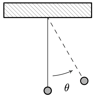

    1. Find a sinusoid which gives the angular displacement \(\theta\) as a function of time, \(t\). Arrange things so \(\theta(0)=\theta_{0}\).

    2. Suppose Sang's Seth-Thomas antique schoolhouse clock needs a period of \(T = \frac{1}{2}\) second and she can adjust the length of the pendulum via a small dial on the bottom of the bob. At what length should she set the pendulum?

    3. Continuing with part (b) and assuming the initial displacement of the pendulum is \(15^{\circ}\), find a sinusoid which models the displacement of the pendulum, \(\theta\), as a function of time, \(t\), in seconds.