5.3: Rigid Transformations

Learning Objectives

• Graph fundamental trigonometric functions having vertical transformations.
• Graph fundamental trigonometric functions having horizontal transformations.
• Graph fundamental trigonometric functions having combinations of all transformations.
• Given the graph, write the corresponding trigonometric function.
• Evaluate given sinusoidal models for applications.
• Build a model for an application based on the graph.

In the previous section, we stated that our ultimate goal (when it comes to graphing the trigonometric functions) is to graph any trigonometric function of the form\[ f(x) = A \, \mathrm{trig}\left( Bx + C \right) + D. \label{unfactoredtrig} \]Now that we know the effect of \( A \) and \( B \) on the graph of the fundamental trigonometric functions, it's time to turn our attention to the parameters \( C \) and \( D \).

Phase Shifts (also known as Horizontal Shifts)

Continuing with alphabetical order, let's focus on the effect of \( C \); however, let's make things simple (for now). Recall¹, the graph of the function\[ y = g(x + C) \nonumber \]is a horizontal shift of the graph of \( g \). It moves the graph to the left \( C \) units if \( C \gt 0 \), and right \( C \) units if \( C \lt 0 \).² Most students in Algebra accept this as truth and memorize the result; however, as you are taking a college-level Trigonometry course, it might serve you well to understand why this is true.

Click here to delve into why the graph of \( y = g(x + C) \) is a horizontal shift of the graph of \( g(x) \)

Well, hello there! I am glad you clicked me! This means you are a natural science person because you investigate truths. Let's start with a simple statement.

Let \( g(x) \) be a function.

Pretty simple, right?

Because \( g \) is a function, each input leads to a single output. Let's grab an arbitrary value from the domain of \( g \) and call it \( x_1 \) (you can call it "happy face" or "star," but \( x_1 \) is easier to write). Again, since \( g \) is a function, \( g\left( x_1 \right) \) must return a single value. Let's call this output \( y_1 \).

So far, all we have said is that \( g \) is a function and that \( g\left( x_1 \right) = y_1 \); however, this last statement means the point \( \left( x_1 , g\left( x_1 \right)\right) \) is on the graph of \( g \).

Now, your friend comes along and says, "Hey, I need to graph \( g\left( x + C \right) \). All I have been given is that \( C \) is positive."

You pause and think for a moment. Turning to your friend, you say, "I don't know what that graph looks like, but I know that when I plug in \( x_1 \) to \( g \), I get out \( y_1 \)."

Your friend smirks and says, "Okay, let's plug \( x_1 \) into \( g\left( x + C \right) \) to find its output!"

You watch him work for a few moments until he gets stuck. He ends up with \( g\left( x_1 + C \right) \), and you look at him quizzically, "I don't know what the value of \( g \) is at \( x_1 + C \). I only know its value at \( x_1 \)."

Then it hits you!

"You did it wrong! You want to evaluate \( g\left( x_1 \right) \). You need to let the argument of your function, which is \( x + C \), be \( x_1 \)."

You start doing the math,\[ x + C = x_1 \implies x = x_1 - C. \nonumber \]You pause... thinking.

"So, to get the argument of \( g\left( x + C \right) \) to be \( x_1 \), we need to plug in \( x_1 - C \) for \( x \)."

Thinking even harder, you have the epiphany.

"With the original function, we plugged in \( x_1 \) and got out \( y_1 \). With \( g\left( x + C \right) \) we needed to plug in \( x_1 - C \) to get \( g\left( x_1 - C + C \right) = g\left( x_1 \right) = y_1\). That is, the original point, \( x_1 \), gets shifted to the left \( C \) units!"

Since our point, \( \left( x_1 , g\left( x_1 \right) \right) \) was arbitrary, all points on the graph of \( g \) experience the same shift. Hence, the graph of \( g\left( x + C \right) \), where \( C \gt 0 \), is the graph of \( g \) shifted \( C \) units to the left.

Example \( \PageIndex{ 1 } \)

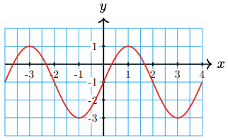
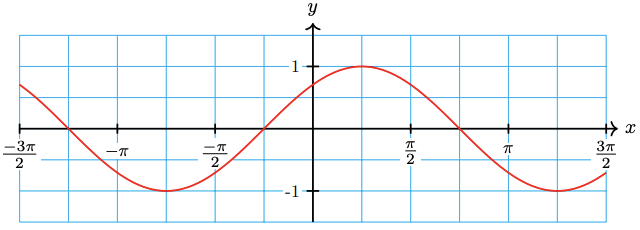
Make a table of values and sketch a graph of \(y=-2 \cos \left(x+\frac{\pi}{3}\right)\).

Solution

From Algebra, we expect the graph to be shifted \(\frac{\pi}{3}\) units to the left compared to the graph of \(y=\cos \left(x\right)\).

As we commonly try to do, we want the argument of \( \cos\left( x + \frac{\pi}{3} \right) \) (which is the expression \( x + \frac{\pi}{3} \)) to be quadrantal angles.

\(x\)	\(x + \dfrac{\pi}{3}\)	\(\cos \left( x + \dfrac{\pi}{3} \right)\)	\(y = 2 \cos \left( x + \dfrac{\pi}{3} \right)\)
	0
	\(\dfrac{\pi}{2}\)
	\(\pi\)
	\(\dfrac{3\pi}{2}\)
	\(2\pi\)

The second column of this table is what we desire \( x + \frac{\pi}{3} \) to be. For \( x + \frac{\pi}{3} \) to become \( 0 \), we solve\[ x + \dfrac{\pi}{3} = 0 \implies x = -\dfrac{\pi}{3}. \nonumber \]Likewise, for \( x + \frac{\pi}{3} \) to become \( \frac{\pi}{2} \), we solve\[ x + \dfrac{\pi}{3} = \dfrac{\pi}{2} \implies x = \dfrac{\pi}{6}. \nonumber \]We continue this process to fill out the first column of the table.

\(x\)	\(x + \dfrac{\pi}{3}\)	\(\cos \left( x + \dfrac{\pi}{3} \right)\)	\(y = 2\cos \left( x + \dfrac{\pi}{3} \right)\)
\(-\dfrac{\pi}{3}\)	0
\(\dfrac{\pi}{6}\)	\(\dfrac{\pi}{2}\)
\(\dfrac{2\pi}{3}\)	\(\pi\)
\(\dfrac{7\pi}{6}\)	\(\dfrac{3\pi}{2}\)
\(\dfrac{5\pi}{3}\)	\(2\pi\)

Finally, we fill out the third and fourth columns using the second column as the arguments.

\(x\)	\(x + \dfrac{\pi}{3}\)	\(\cos \left( x + \dfrac{\pi}{3} \right)\)	\(y = 2\cos \left( x + \dfrac{\pi}{3} \right)\)
\(-\dfrac{\pi}{3}\)	0	1	-2
\(\dfrac{\pi}{6}\)	\(\dfrac{\pi}{2}\)	0	0
\(\dfrac{2\pi}{3}\)	\(\pi\)	-1	2
\(\dfrac{7\pi}{6}\)	\(\dfrac{3\pi}{2}\)	0	0
\(\dfrac{5\pi}{3}\)	\(2\pi\)	1	-2

We now plot the \( x \)-values (in the first column) and their corresponding function values (in the fourth column) to make the graph. One cycle of the graph is shown below. As we expected,the graph is shifted \(\frac{\pi}{3}\) units to the left compared to the graph of \(y=-2\cos \left(x\right)\).

Checkpoint \( \PageIndex{ 1 } \)

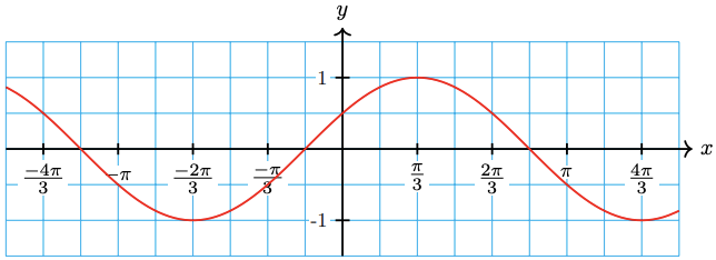
Complete the table and sketch a graph of \(y=-3\sin \left(x-\frac{\pi}{6}\right)\). (Do you expect the graph to be shifted to the left or the right, compared to the graph of \(y=-3\sin \left(x\right) \)?)

\(x\)	\(x - \dfrac{\pi}{6}\)	\(\sin \left( x - \dfrac{\pi}{6} \right)\)	\(y = -3 \sin \left( x - \dfrac{\pi}{6} \right)\)
	0
	\(\dfrac{\pi}{2}\)
	\(\pi\)
	\(\dfrac{3\pi}{2}\)
	\(2\pi\)

Answer

\(x\)	\(x - \dfrac{\pi}{6}\)	\(\sin \left( x - \dfrac{\pi}{6} \right)\)	\(y = -3 \sin \left( x - \dfrac{\pi}{6} \right)\)
\(\dfrac{\pi}{6}\)	0	0	0
\(\dfrac{2\pi}{3}\)	\(\dfrac{\pi}{2}\)	1	-3
\(\dfrac{7\pi}{6}\)	\(\pi\)	0	0
\(\dfrac{5\pi}{3}\)	\(\dfrac{3\pi}{2}\)	-1	3
\(\dfrac{13\pi}{6}\)	\(2\pi\)	0	0

Example \( \PageIndex{ 1 } \) and Checkpoint \( \PageIndex{ 1 } \) should convince you that our previous experience from Algebra with horizontal shifts of functions still works with trigonometric functions; however, let's solidify that concept to drive the point home.

We know that all the fundamental trigonometric functions have principal cycles occurring on the interval \( 0 \leq \theta \leq p \), where \( \theta \) is the argument and \( p \) is the function's natural period. This means that the modified function\[ f(x) = \mathrm{trig}\left( x + C \right) \nonumber \]goes through that same cycle when \( 0 \leq x + C \leq p \). Subtracting \( C \) from all three sides, we discover that this modified trigonometric function goes through the same single cycle on the interval \( -C \leq x \leq p - C \). That is, the starting point for the principal cycle has been shifted from \( 0 \) to \( -C \). This shift in the starting point from the principal cycle is known as the phase shift of the trigonometric function. This definition is so important that we should codify it.

Definition: Phase Shift

The phase shift of a trigonometric function is the \( x \)-value of where the initial number in the principal cycle has been shifted.

Thus, the phase shift for the function in Example \( \PageIndex{ 1 } \) is \( - C = -\frac{\pi}{3} \) and the phase shift for the function in Checkpoint \( \PageIndex{ 1 } \) is \( -C = -\left(-\frac{\pi}{6}\right) = \frac{\pi}{6} \).

This gets us to the point where we can expertly graph a trigonometric function of the form\[ f(x) = A \, \mathrm{trig}\left( x + C \right), \nonumber \]but what happens when the coefficient of \( x \) is not \( 1 \)? That is, if we are given\[ f(x) = A \, \mathrm{trig}\left( Bx + C \right), \nonumber \]is the phase shift still \( -C \)?

The answer to this question is an adamant no.

Using our previous derivation, the modified function\[ f(x) = A \, \mathrm{trig}\left( Bx + C \right) \nonumber \]goes through its principal cycle when \( 0 \leq Bx + C \leq p \), where \( p \) is the natural period of the trigonometric function. Subtracting \( C \) from all three sides, we get \( -C \leq Bx \leq p - C \). Assuming \( B \gt 0 \), we can divide all three sides by \( B \) to find that this modified trigonometric function goes through the same single cycle on the interval \( -\frac{C}{B} \leq x \leq \frac{p - C}{B} \). That is, the starting point for the principal cycle has been shifted from \( 0 \) to \( -\frac{C}{B} \). Therefore, the phase shift is \( -\frac{C}{B} \). The following theorem summarizes all of this into a nice, clean statement.

Theorem: Phase Shift of \( y = A \, \mathrm{trig}\left( Bx + C \right) \)

The phase shift of the function\[ y = A \, \mathrm{trig}\left( Bx + C \right) \nonumber \]is \( -\frac{C}{B} \).

By the way, if \( B \lt 0 \), we do what we did in the last section and use the Symmetry Identities to force it to become positive.

Before going through some examples, it's best to issue a caution.

Caution: \( C \) is Not Always the Phase Shift

When considering the function\[ f(x) = A \, \mathrm{trig}\left( Bx + C \right), \nonumber \]it is crucial to remember that \( B \) is not the period and \( C \) is not necessarily the phase shift.³

• \( \text{Period} = \dfrac{2\pi}{B} \)
• \( \text{Phase Shift} = -\dfrac{C}{B} \)

Example \(\PageIndex{2}\)

State the phase shift of each function.

1. \( y = 2 \tan\left( 6x - \pi \right) \)
2. \( y = \sqrt{5} \sin\left( -\frac{\pi}{2}x + \frac{\pi}{4} \right) \)

Solutions

1. In this case, \( B = 6 \) and \( C = -\pi \). Hence, the phase shift for this function is\[ -\dfrac{C}{B} = -\dfrac{-\pi}{6} = \dfrac{\pi}{6}. \nonumber \]
2. As in the previous section, we must use the Symmetry Identities when \( B \lt 0 \). When using these identities, be sure to factor the negative off both \( B \) and \( C \).\[ \begin{array}{rclcr}
   y & = & \sqrt{5} \sin\left( -\dfrac{\pi}{2}x + \dfrac{\pi}{4} \right) & \quad & \\
   & = & \sqrt{5} \sin\left( -\left( \dfrac{\pi}{2}x - \dfrac{\pi}{4} \right) \right) & & \\
   & = & -\sqrt{5} \sin \left( \dfrac{\pi}{2}x - \dfrac{\pi}{4} \right) & & \left( \text{sine is an odd function} \right) \\
   \end{array} \nonumber \]Hence, the phase shift is\[ -\dfrac{C}{B} = - \dfrac{-\pi/4}{\pi/2} = \dfrac{\pi}{2}.\nonumber \]

Checkpoint \(\PageIndex{2}\)

State the phase shift of \(y=-2 \cos \left(2 x - \frac{\pi}{3}\right)\)

Answer

\( \dfrac{\pi}{6} \)

Some instructors (including myself) introduce an alternative way of manipulating the argument of the trigonometric function \( f(x) = A\,\mathrm{trig}\left( Bx + C \right) \). If you factor \( B \) from all terms in the argument, your function turns into\[ f(x) = A \, \mathrm{trig}\left( B\left( x + \dfrac{C}{B} \right) \right). \nonumber \]In this form, the phase shift reveals itself because \( \frac{C}{B} = - \left( -\frac{C}{B} \right) \) and so\[ f(x) = A\,\mathrm{trig}\left( B\left( x - \left( -\dfrac{C}{B} \right) \right) \right). \nonumber \]We will include this in an example or two, just in case your instructor likes this form.

We now modify our graphing tactic from the previous section to include this new transformation.

Summary of Graphing \( f(x) = \overline{A} \, \mathrm{trig}\left( \overline{B}x + \overline{C}\right) \)

To graph the function\[ f(x) = \overline{A} \, \mathrm{trig}\left( \overline{B}x + \overline{C}\right): \nonumber \]

Precondition Stage

We begin by cleaning up the trigonometric function and ensuring that the coefficient of \( x \) is positive. This is done using the Symmetry Identities. Again, as a warning, if \( \overline{B} \lt 0 \), you will factor a negative off both terms in the argument of the trigonometric function. Once the Symmetry Identities have been used, your new function will be of the form\[ f(x) = A \, \mathrm{trig}\left( Bx + C\right). \nonumber \]

Information Stage

We now identify the following information (in the order listed):

• \( \text{Amplitude} = \left| A \right| \)
• \( \text{Period} = \dfrac{\text{Natural Period}}{B} \)
• \( \text{Step Size} = \dfrac{\text{Period}}{4} \)
• \( \text{Phase Shift} = - \dfrac{C}{B} \)

where the natural period is \( 2\pi \) if given the sine or cosine functions, and \( \pi \) if given the tangent function.

Graphing Stage

We then use each of these in reverse order to obtain a sketch of the trigonometric function.

• Draw a horizontal line and mark the initial key number as the phase shift.
• Mark the remaining key numbers by successively adding the step size to the previous key number.
• Double-check that the distance from the initial key number to the final key number matches the period, then sketch one cycle of the base trigonometric function, making sure to account for the sign of \( A \) and drawing any vertical asymptotes (if the given function is the tangent).
• Draw the vertical axis at \( x = 0 \) and use the amplitude to either
  • label the maximum and minimum values of the trigonometric function on the vertical axis (if the given function is sinusoidal), or
  • label the remaining key points on the graph (if the given function is the tangent).

Example \(\PageIndex{3}\)

Graph a single cycle of the given trigonometric function, labeling key numbers, the \( y \)-axis, stating the period, step size, amplitude, and phase shift.

1. \( y = 2 \tan\left( 6x - \pi \right) \)
2. \( y = \sqrt{5} \sin\left( -\frac{\pi}{2}x + \frac{\pi}{4} \right) \)

Solutions

1. Precondition Stage: Since \( B = 6 \gt 0 \), there is nothing to precondition; however, if we wanted to factor the \( 6 \) from both terms in the argument, we would get\[ y = 2 \tan\left( 6\left( x - \frac{\pi}{6} \right) \right), \nonumber \]which reveals the phase shift to be \( \frac{\pi}{6} \).
   Information Stage: This is not a sinusoidal function, so we will not have an amplitude, and the natural period is \( \pi \). \[ \begin{array}{rclcrcl}
   \hline B & = & 6 & \implies & \text{Period} & = & \dfrac{\text{Natural Period}}{B} = \dfrac{\pi}{6} \\
   \hline \quad & \quad & \quad & \implies & \text{Step Size} & = & \dfrac{\text{Period}}{4} = \dfrac{\pi/6}{4} = \dfrac{\pi}{24} \\
   \hline C & = & -\pi & \implies & \text{Phase Shift} & = & - \dfrac{C}{B} = - \dfrac{-\pi}{6} = \dfrac{\pi}{6} = \dfrac{4\pi}{24} \\
   \hline \end{array} \nonumber \]It's a good idea to get the phase shift and the step size to have the same denominator, as you will add the step size to the phase shift in the graphing stage.
   Graphing Stage: Graphing a number line (the \( x \)-axis), we plot the phase shift and, from there, mark the remaining key numbers using the step size.

   

   The distance between the initial key number and the final key number is\[ \left| \dfrac{8\pi}{24} - \dfrac{4\pi}{24} \right| = \dfrac{4\pi}{24} = \dfrac{\pi}{6} = \text{Period} \nonumber \]so we have done well so far. We now sketch a single cycle of the unreflected tangent function, drawing in the vertical asymptote halfway through the cycle.

   

   We can see that the initial key number is positive and, therefore, to the right of the \( y \)-axis. Consequently, we draw in the \( y \)-axis where we think it should be. Simultaneously, let's plot the points corresponding to the key numbers \( \frac{5\pi}{24} \) and \( \frac{7\pi}{24} \).

   

   This completes one full cycle of the graph of the given function (although we decided to show some extra cycles, it's not a requirement).
2. Precondition Stage: Since \( B = -\frac{\pi}{2} \lt 0 \), we need to factor a negative from both terms in the argument of the function.\[ \begin{array}{rclcr}
   y & = & \sqrt{5} \sin\left( -\dfrac{\pi}{2}x + \dfrac{\pi}{4} \right) & \quad & \\
   & = & \sqrt{5} \sin\left( -\left(\dfrac{\pi}{2}x - \dfrac{\pi}{4}\right) \right) & & \\
   & = & -\sqrt{5} \sin\left( \dfrac{\pi}{2}x - \dfrac{\pi}{4} \right) & & \left( \text{sine is an odd function} \right) \\
   \end{array} \nonumber \]Moreover, if your instructor prefers the factored form, we could factor the \( \frac{\pi}{2} \) from both terms in the argument to get\[ y = -\sqrt{5} \sin\left( \dfrac{\pi}{2} \left( x - \dfrac{1}{2} \right) \right). \nonumber \]Doing this reveals the phase shift to be \( \frac{1}{2} \).
   Information Stage: This is a sinusoidal function, so we will have an amplitude, and the natural period is \( 2 \pi \). \[ \begin{array}{rclcrcl}
   \hline A & = & -\sqrt{5} & \implies & \text{Amplitude} & = & \left| A \right| = \left| -\sqrt{5} \right| = \sqrt{5} \\
   \hline B & = & \dfrac{\pi}{2} & \implies & \text{Period} & = & \dfrac{\text{Natural Period}}{B} = \dfrac{2 \pi}{\pi/2} = 4 \\
   \hline \quad & \quad & \quad & \implies & \text{Step Size} & = & \dfrac{\text{Period}}{4} = \dfrac{4}{4} = 1 \\
   \hline C & = & -\frac{\pi}{4} & \implies & \text{Phase Shift} & = & - \dfrac{C}{B} = - \dfrac{-\pi/4}{\pi/2} = \dfrac{1}{2} \\
   \hline \end{array} \nonumber \]
   Graphing Stage: It's important to remember that we are graphing the "cleaned" function\[ y = -\sqrt{5} \sin\left( \dfrac{\pi}{2}x - \dfrac{\pi}{4} \right). \nonumber \]Graphing the \( x \)-axis, plotting the phase shift, and marking the subsequent key numbers by increasing by the step size, we get the following:

   

   We then graph the reflected sine function.

   

   Finally, we place the \( y \)-axis appropriately, label it using the amplitude, and label the maximum and minimum points on the sine curve (this is something we didn't do before, but some instructors expect it, so we want to showcase good behavior).

   

Checkpoint \(\PageIndex{3}\)

Graph \(y=-2 \cos \left(2 x+\frac{\pi}{3}\right)\) and state the period, amplitude, step size, and phase shift.

Answer

Amplitude: \( 2 \)
Period: \( \pi \)
Step Size: \( \frac{\pi}{4} \)
Phase Shift: \( -\frac{\pi}{6} \)

As we have done previously, you can use the following Interactive Element to help visualize the effect of \( C \) on the graph of the sine function.

Interactive Element: Investigating the Effects of \( C \) on the Graph of \( y = A \, \sin\left( Bx + C \right) \)

Interaction: Adjust the slider for \( A \), \( B \), and \( C \) to see the effect on the graph of \(y = A \, \sin\left(Bx + C\right)\).

Vertical Shifts and the Midline

We finish our discussion of transformations with the parameter \( D \) in the function\[ f(x) = A \, \mathrm{trig}\left( Bx + C \right) + D. \nonumber \]Of all the transformations from your Algebra class, this is the one most students are pretty good with. Recall, the graph of \[ y = g(x) + D \nonumber \]is the graph of \( g \) shifted up (if \( D \gt 0 \)) or down (if \( D \lt 0 \)) \( |D| \) units. That is, the "\( + D \)" is just adding \( D \) to all the \( y \)-values of the original function.

The only new concept here is the idea of a midline for a trigonometric function. Prior to rigid transformations, the base trigonometric function is built solely along the \( x \)-axis; however, once a vertical shift occurs, a "hidden" axis appears. This axis is called the "midline," and it is handy when graphing trigonometric functions.

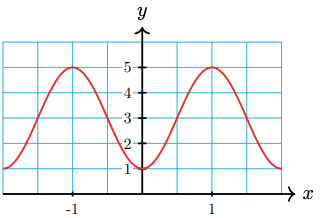
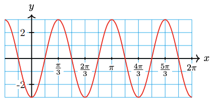
For example, consider the function\[ y = -2 \sin\left( \pi x \right) + 3. \nonumber \]From the previous section, we should be able to quickly sketch most of this function, but the "\( + 3 \)" at the end is new. We know the base function is the sine, the fact that the coefficient of the sine is negative means the base graph has been reflected about the \( x \)-axis, the amplitude (because the graph is sinusoidal) is \( |-2| = 2 \), the period is \( \frac{2 \pi}{B} = \frac{2 \pi}{\pi} = 2 \), and the step size is \( \frac{\text{Period}}{4} = \frac{2}{4} = \frac{1}{2} \). If this is all we had, then the graph would look like the following:

Figure \( \PageIndex{ 1 } \): \( y = -2 \sin\left( \pi x \right) \)

Since our given function is\[ y = -2 \sin\left( \pi x \right) + 3, \nonumber \]we need to add three to all of the outputs in Figure \( \PageIndex{ 1 } \).⁴ As we redraw our graph and shift up three units, it is helpful to move up the hidden midline.

Figure \( \PageIndex{ 2 } \): \( y = -2 \sin\left( \pi x \right) + 3\)

Let's update our graphing tactic a final time.

Summary of Graphing \( f(x) = \overline{A} \, \mathrm{trig}\left( \overline{B}x + \overline{C}\right) + D\)

To graph the function\[ f(x) = \overline{A} \, \mathrm{trig}\left( \overline{B}x + \overline{C}\right) + D: \nonumber \]

Precondition Stage

• If the trigonometric function is not written in the order listed above (e.g. if you are given \( y = 3 - 2 \sin\left( 5 - x \right) \)), rewrite it so it matches the form above - this is critical!
• Clean up the trigonometric function using the Symmetric Identities to ensure the coefficient of \( x \) is positive. Again, as a warning, if \( \overline{B} \lt 0 \), you will factor a negative off both terms in the argument of the trigonometric function. Once the Symmetry Identities have been used, your new function will be of the form\[ f(x) = A \, \mathrm{trig}\left( Bx + C\right) + D. \nonumber \]

Information Stage

We now identify the following information (in the order listed):

• \( \text{Amplitude} = \left| A \right| \)
• \( \text{Period} = \dfrac{\text{Natural Period}}{B} \)
• \( \text{Step Size} = \dfrac{\text{Period}}{4} \)
• \( \text{Phase Shift} = - \dfrac{C}{B} \)
• \( \text{Vertical Shift} = D \)

where the natural period is \( 2\pi \) if given the sine or cosine functions, and \( \pi \) if given the tangent function.

Graphing Stage

We then use each of these in reverse order to obtain a sketch of the trigonometric function.

• Draw a horizontal line and label it \( y = D \). This is your vertical shift.
• Mark the initial key number as the phase shift
• Mark the remaining key numbers by successively adding the step size to the previous key number.
• Double-check that the distance from the initial key number to the final key number matches the period, then sketch one cycle of the base trigonometric function, making sure to account for the sign of \( A \) and drawing any vertical asymptotes (if the given function is the tangent).
• Draw the vertical axis at \( x = 0 \) and use the amplitude to either
  • label the maximum and minimum values of the trigonometric function on the vertical axis (if the given function is sinusoidal), or
  • label the remaining key points on the graph (if the given function is the tangent).

Example \(\PageIndex{4}\)

Graph each function. State the amplitude (if applicable), period, step size, phase shift, and vertical shift. Your graph should have five key points (or four key points and an asymptote) labeled, as well as the midline.

1. \( y = -5 + 5\sin\left( 3 \pi x + \frac{\pi}{2} \right)\)
2. \( y = \frac{1}{3} \tan\left( 2x - 1 \right) + 1 \)

Solutions

1. Precondition Stage: Rewriting the given function into proper form, we get\[ y = 5\sin\left( 3 \pi x + \dfrac{\pi}{2} \right) - 5. \nonumber \]Information Stage:\[ \begin{array}{rclcrcl}
   \hline A & = & 5 & \implies & \text{Amplitude} & = & 5 \\
   \hline B & = & 3 \pi & \implies & \text{Period} & = & \dfrac{\text{Natural Period}}{B} = \dfrac{2 \pi}{3 \pi} = \dfrac{2}{3} \\
   \hline \quad & \quad & \quad & \implies & \text{Step Size} & = & \dfrac{\text{Period}}{4} = \dfrac{2/3}{4} = \dfrac{1}{6} \\
   \hline C & = & \dfrac{\pi}{2} & \implies & \text{Phase Shift} & = & - \dfrac{C}{B} = - \dfrac{\pi/2}{3 \pi} = -\dfrac{1}{6} \\
   \hline D & = & -5 & \implies & \text{Vertical Shift} & = & -5 \\
   \hline \end{array} \nonumber \]That last line tells us the midline is \( y = -5 \).
   Graphing Stage: We start by graphing a horizontal line and labeling it \( y = -5 \).

   

   We then plot five equally-spaced points, labeling the first using the phase shift, and adding the step size to reach each subsequent point.

   

   Double-checking the length of the interval, we see that\[ \left| \dfrac{3}{6} - \left( -\dfrac{1}{6} \right)\right| = \dfrac{4}{6} = \dfrac{2}{3} = \text{Period}. \nonumber \]So far, so good! The function we want to graph is an unreflected sine function, so let's use these key numbers to sketch.

   

   From here, we can see where \( x = 0 \) is, so we know where the \( y \)-axis goes.

   

   Since the midline is at \( y = -5 \) and the amplitude is \( 5 \), we can label the \( y \)-axis by adding and subtracting the amplitude from the midline.

   

   Finally, now that we see where \( y = 0 \), we can draw the \( x \)-axis.

   

   That is a complete cycle of the graph of \( y = -5 + 5\sin\left( 3 \pi x + \frac{\pi}{2} \right)\).
2. Precondition Stage: There is nothing to precondition here.
   Information Stage: \[ \begin{array}{rclcrcl}
   \hline B & = & 2 & \implies & \text{Period} & = & \dfrac{\text{Natural Period}}{B} = \dfrac{\pi}{2} \\
   \hline \quad & \quad & \quad & \implies & \text{Step Size} & = & \dfrac{\text{Period}}{4} = \dfrac{\pi/2}{4} = \dfrac{\pi}{8} \\
   \hline C & = & -1 & \implies & \text{Phase Shift} & = & - \dfrac{C}{B} = - \dfrac{-1}{2} = \dfrac{1}{2} \\
   \hline D & = & 1 & \implies & \text{Vertical Shift} & = & 1 \\
   \hline \end{array} \nonumber \]This is a case where the phase shift (\( \frac{1}{2} \)) and the step size (\( \frac{\pi}{8} \)) are not easily added together. Please pay close attention to how we handle this during the graphing stage.
   Graphing Stage: Graph the midline, plot five equally-spaced points, call the first point the phase shift, and label the remaining using the step size.

   

   We now graph the unreflected tangent function and graph the vertical asymptote in the middle of the cycle. Moreover, we place the \( y \)-axis.

   

   We can see that two of our key points are "labeled" (\( \left( \frac{1}{2},1 \right) \) and \( \left( \frac{1}{2} + \frac{4\pi}{8},1 \right) \)) and we have the asymptote labeled (\( x = \frac{1}{2} + \frac{2 \pi}{8} \)); however, we have two extra key numbers that need to be used. Despite the tangent function not having an amplitude, \( |A| = \frac{1}{3} \) still serves a purpose. It tells us how far away from the midline the points corresponding to those unlabeled key numbers should be. That is, the \( y \)-value associated with \( x = \frac{1}{2} + \frac{\pi}{8} \) is \( 1 + \frac{1}{3} = \frac{4}{3} \). Likewise, the \( y \)-value for \( x = \frac{1}{2} + \frac{3\pi}{8} \) is \( 1 - \frac{1}{3} = \frac{2}{3} \). We label these points and draw in the \( x \)-axis (appropriately).

   

Checkpoint \(\PageIndex{4}\)

Graph the function. State the amplitude (if applicable), period, step size, phase shift, and vertical shift. Your graph should have five key points (or four key points and an asymptote) labeled, as well as the midline.\[ f(x) = 3 -\frac{7}{5} \tan\left( 2x - \dfrac{\pi}{2} \right) \nonumber \]

Answer

Period: \( \frac{\pi}{2} \)
Step Size: \( \frac{\pi}{8} \)
Phase Shift: \( \frac{\pi}{4} \)
Vertical Shift: \( 3 \)

Interactive Element: Ivestigating the Effects of \( D \) on the Graph of \( y = A \, \sin\left( Bx + C \right) + D \)

Interaction: Adjust the sliders for each parameter to see the effects on the graph of \( y = A \sin\left( Bx + C \right) + D \).

Finding Equations Given Graphs

Finding the equation of a trigonometric function given its graph is only slightly more complex when there has been a phase shift or vertical shift. The key to success with these problems is identifying two points on the curve. This is usually enough to find the equation.

Example \(\PageIndex{5}\)

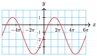
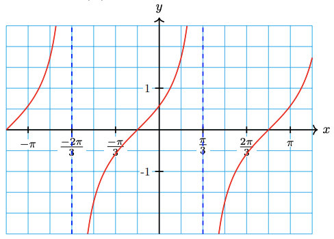
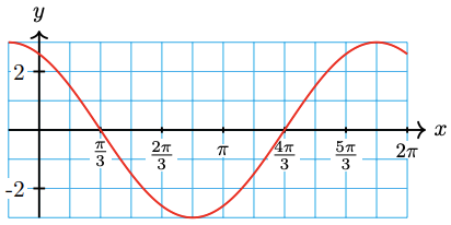
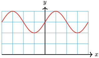
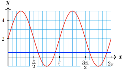
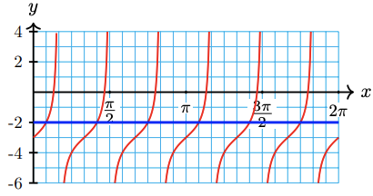
Find the equation of the graphed function.

1. 
2. 

Solutions

1. When rebuilding an equation from a graph, it's best to figure out the information using the order with which we graph. That is, try to identify the vertical shift, phase shift, period (which might require finding the step size), and amplitude (if applicable). This is more of a "rule of thumb," so there might be times you do things out of order.
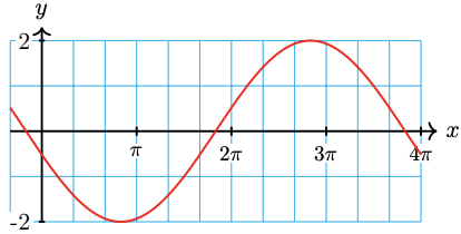
   Vertical Shift: Since the maximum and minimum of this sinusoidal function are \( -\frac{1}{2} \) and \( -\frac{3}{2} \), respectively, the midline must sit directly between these two values. That is, the vertical shift is the average of these.\[ \text{Vertical Shift} = D = \dfrac{-\frac{1}{2} + \left( -\frac{3}{2} \right)}{2} = -1. \nonumber \]Phase Shift: Given the graph of a sinusoidal function and asked to find the equation, you have a lot of options. For example, the given graph could be interpreted as a sine function shifted slightly to the left (or slightly to the right and reflected about \( y = -1 \)); however, try to use the given information to make the process easier. We will assume the leftmost point we were given, \( \left( -\frac{5\pi}{18}, - \frac{3}{2} \right) \), is the phase shift. Thus,\[ \text{Phase Shift} = -\dfrac{C}{B} = -\dfrac{5\pi}{18}. \label{ex5a} \]While this does not immediately give us \( B \) or \( C \), it does tell us that we are dealing with a reflected cosine function. We will use Equation \ref{ex5a} in a moment.
   Period or Step Size: Assuming the cycle begins at \( x = -\frac{5\pi}{18} \), we can see that the curve is halfway through a full cycle by \( x = \frac{\pi}{18} \). That is, half the period is \( \left| -\frac{5\pi}{18} - \frac{\pi}{18} \right| = \frac{6\pi}{18} = \frac{\pi}{3} \). Therefore, the full period is \( \frac{2\pi}{3} \), and so\[ \text{Period} = \dfrac{2\pi}{B} = \frac{2\pi}{3} \implies B = 3. \nonumber \]We can now go back to Equation \ref{ex5a} and let \( B = 3 \) to get\[ -\dfrac{C}{3} = -\dfrac{5 \pi}{18} \implies C = \dfrac{5 \pi}{6}. \nonumber \]Amplitude: The amplitude is the distance from the midline to the maximum (or minimum). In this case, the amplitude is\[ \text{Amplitude} = |A| = \dfrac{1}{2}. \nonumber \]Putting this altogether, and remembering that the function is a reflected cosine function, we get\[ f(x) = -\dfrac{1}{2} \cos\left( 3x + \dfrac{5\pi}{6} \right) - 1. \nonumber \]It's crucial for me to state that there are an infinite number of current answers when it comes to stating the equation of a trigonometric function. If checking your work against a friend's work and if your friend has a different function, you should graph both equations to see if they are equivalent.
2. Vertical Shift: If you imagine a horizontal midline for this tangent-like curve, it would be at \( y = 1 \). Thus,\[ D = 1. \nonumber \]Phase Shift: Remember that the principal cycle of the tangent function starts at the midline (\( x \)-axis). Thus, we will assume the first point, \( \left( 1,1 \right) \), is where the cycle of this shifted function starts. This means the function is a reflected tangent function and \[ \text{Phase Shift} = -\dfrac{C}{B} = 1. \label{ex5b} \]Period or Step Size: The tangent is a nice function to deal with sometimes because we can see the period from the vertical asymptotes. The distance between these matches the period of the given tangent function. Therefore,\[ \text{Period} = \dfrac{\pi}{B} = |2.5 - (-0.5) | = 3 \implies B = \frac{\pi}{3}. \nonumber \]Pluggin this back into Equation \ref{ex5b}, we get\[ -\dfrac{C}{\pi/3} = 1 \implies C = -\dfrac{\pi}{3}. \nonumber \]Amplitude: Since we are dealing with a tangent function, there is no amplitude, but we still need to determine the coefficient of the tangent function. Luckily, we were given a second point, \( \left( \frac{7}{4}, -1 \right) \). So far we have\[ g(x) = A \tan\left( Bx + C \right) + D = A \tan\left( \dfrac{\pi}{3}x - \dfrac{\pi}{3} \right) + 1. \nonumber \]Letting the output be \( -1 \) and \( x = \frac{7}{4} \), we get\[ \begin{array}{rrcl}
   & -1 & = & A \tan\left( \dfrac{7\pi}{12} - \dfrac{\pi}{3} \right) + 1 \\
   \implies & -2 & = & A \tan\left( \dfrac{7\pi}{12} - \dfrac{4\pi}{12} \right) \\
   \implies & -2 & = & A \tan\left( \dfrac{3\pi}{12} \right) \\
   \implies & -2 & = & A \tan\left( \dfrac{\pi}{4} \right) \\
   \implies & -2 & = & A(1) \\
   \implies & -2 & = & A \\
   \end{array} \nonumber \]Hence,\[ g(x) = -2 \tan\left( \dfrac{\pi}{3}x - \dfrac{\pi}{3} \right) + 1. \nonumber \]

Checkpoint \(\PageIndex{5}\)

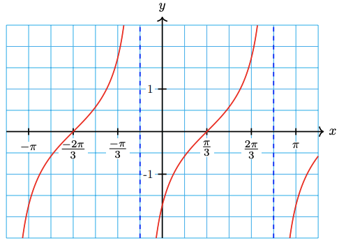
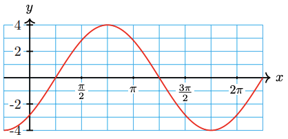
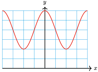
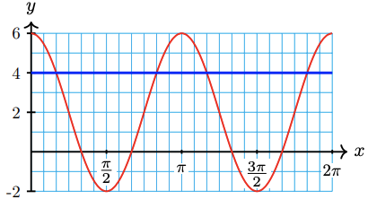
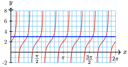
Find the equation of the graphed function.

Answer

\( y = 3\sin\left( 2x + \frac{\pi}{4} \right) - 1\)

Revisiting the Cofunction Identities

Recall from section 3.1, the Cofunction Identities (which we rewrite here in radian measure).

Theorem: Cofunction Identities

The trigonometric function of an angle is equal to the cofunction evaluated at the complement of the angle. That is,\[ \begin{array}{rcccccccl}
\sin\left( \theta \right) & = & \cos\left( \dfrac{\pi}{2} - \theta \right) & \quad & \text{and} & \quad & \cos\left( \theta \right) & = & \sin\left( \dfrac{\pi}{2} - \theta \right) \\
\sec\left( \theta \right) & = & \csc\left( \dfrac{\pi}{2} - \theta \right) & \quad & \text{and} & \quad & \csc\left( \theta \right) & = & \sec\left( \dfrac{\pi}{2} - \theta \right) \\
\tan\left( \theta \right) & = & \cot\left( \dfrac{\pi}{2} - \theta \right) & \quad & \text{and} & \quad & \cot\left( \theta \right) & = & \tan\left( \dfrac{\pi}{2} - \theta \right) \\
\end{array} \nonumber \]

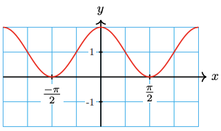
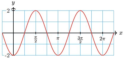
At the time, we could only prove these identities for acute angles. We are still not at a point where we can prove these for all angles, but we can now visualize these identities. For example, let's consider the function \( y = \cos\left( \frac{\pi}{2} - x \right) \). The Cofunction Identities tell us that this should be the same as \( y = \sin\left( x \right) \). Let's manipulate that cosine function a little.\[ \begin{array}{rclcc}
y & = & \cos\left( \frac{\pi}{2} - x \right) & \quad & \\
& = & \cos\left( -\left( - \frac{\pi}{2} + x \right) \right) & & \\
& = & \cos\left( -\left( x - \frac{\pi}{2} \right) \right) & & \\
& = & \cos\left( x - \frac{\pi}{2} \right) & & \left( \text{cosine is an even function} \right) \\
\end{array} \nonumber \]So, that cosine function is just like a regular cosine function, but with a phase shift of \( \frac{\pi}{2} \). Graphing this, we get the following:

However, this is exactly the graph of \( y = \sin\left( x \right) \). Therefore, we feel confident in stating that \( \cos\left( \frac{\pi}{2} - x \right) = \sin\left( x \right) \). You can use the same technique to convince yourself that the other Cofunction Identities are true (go ahead, it's a great exercise!).

Introduction to Sinusoidal Models

Many natural phenomena can be modeled with sinusoidal functions. In this subsection, we will work with applications where we have either been given the explicit sinusoidal model or the graph that models a situation. In the next section, we will learn to build sinusoidal models from language.

Example \( \PageIndex{ 6 } \)

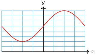
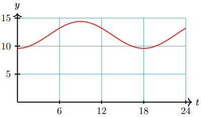
The formula\[D(t)=12.25-5.25 \cos \left(\dfrac{\pi}{6} t\right)\nonumber \]gives the number of hours of daylight in Glasgow, Scotland, as a function of time, in months after January 1.

1. Graph the function by hand.
2. State the midline, amplitude, and period of the graph.
3. How many hours of daylight does Glasgow enjoy on the longest day of the year?
4. In which months does Glasgow experience less than 8 hours of light daily?

Solutions

1. We begin by rewriting the function as\[ D(t) = -5.25\cos\left( \dfrac{\pi}{6} t \right) + 12.25. \nonumber \]The amplitude is \( A = 5.25 \), the period is \( \frac{2\pi}{\pi/6} = 12 \). Therefore, the step size is \( 3 \). Since \( C = 3 \), there is no phase shift. Finally, the vertical shift is \( 12.25 \). Graphing the reflected cosine starting at \( t = 0 \), stepping by \( 3 \), with an amplitude of \( 5.25 \), we get the following graph.

   

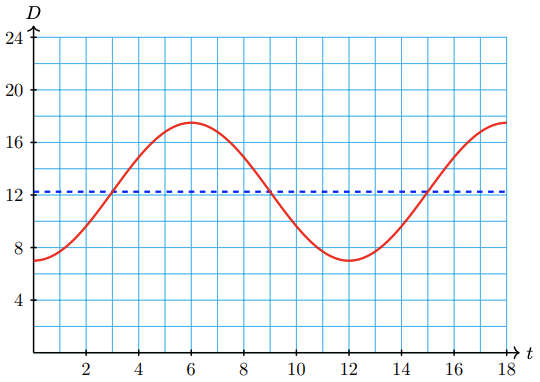
2. The midline of the graph is \(D\) = 12.25 hours, the amplitude is 5.25 hours, and the period is 12 months.
3. On the longest day of the year, there are 12.25 + 5.25 = 17.5 hours of daylight in Glasgow.
4. From the graph, we see that \(D(t)<8\) for \(t\) between 0 and 2, or in January and February. \(D(t)\) is also less than 8 for a short time between \(t=11\) and \(t=12\) at the end of December.

Checkpoint \( \PageIndex{ 6 } \)

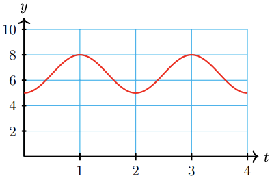
The pistons in an automobile engine move up and down in the cylinders. If \(t\) is in milliseconds, the distance from the top of the piston to the top of the cylinder is given in centimeters by\[D=7+6 \sin (4 \pi t)\nonumber \]

1. Graph the function by hand.
2. State the midline, amplitude, and period of the graph.
3. Find the largest and the smallest clearance between the piston and the top of the cylinder.

Answer

1. 
2. Midline: \(D=7\), amplitude: 6 , period: \(0.5 \mathrm{millisec}\)
3. Largest: \(13 \mathrm{~cm}\), smallest: \(1 \mathrm{~cm}\)

Example \( \PageIndex{ 7 } \)

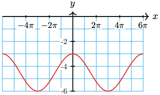
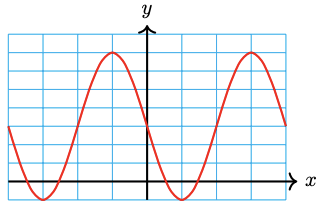
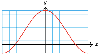
Sunspots are dark regions on the Sun first observed by Galileo in 1610. The number of sunspots is not constant but varies with a period of approximately 11 years, called the solar cycle. Solar activity is directly related to this cycle and can cause disturbances in the Earth’s upper atmosphere. Planning for satellite orbits and space missions requires knowledge of solar activity levels years in advance.

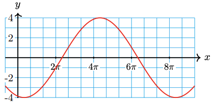
The figure below shows sunspot data for the last solar cycle, from July 1985 through June 1996, and a sinusoidal function that models the data.

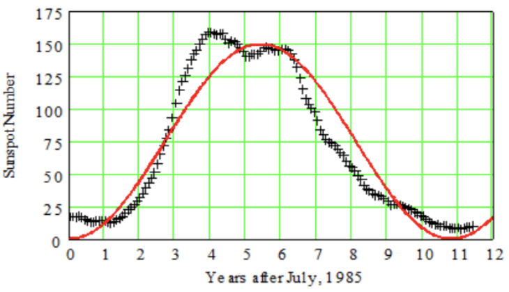
The period of the solar cycle shown is 10.8 years. Use this information and the graph to write a formula for the model.

Solution

The graph has the shape of \(y=-\cos \left(x\right)\). It appears to have midline \(y=75\) and amplitude 75, so \(|A|=75\) and \(A=-75\). To find \(B\), we compute\[\text{Period} = \dfrac{2\pi}{B} \implies B=\dfrac{2 \pi}{\text {Period}}=\dfrac{2 \pi}{10.8} \approx 0.58\nonumber \]Thus, a formula for the model is\[y = -75 \cos \left(0.58x + C\right)] + 75.\nonumber \]If we are trying to fit the red curve, the phase shift would be \( 0 \) and so \( C = 0 \).Hence,\[ y = -75 \cos\left( 0.58x \right) + 75. \nonumber \]

Checkpoint \( \PageIndex{ 7 } \)

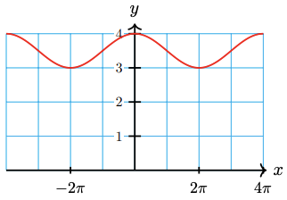
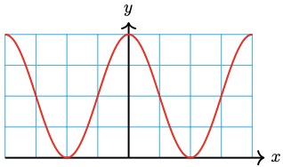
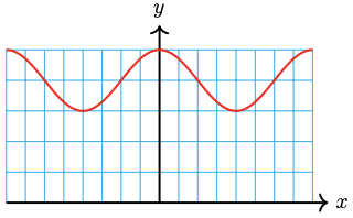
The figure below shows the sunspot data for the solar cycle that began in July 1996, and a curve of best fit calculated by NASA. This curve is not sinusoidal, but has a similar shape.

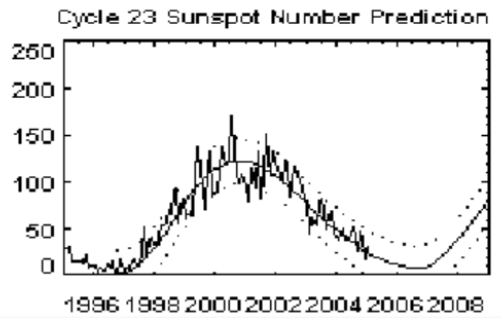
1. The minimum sunspot number occurred in October 1996. Use the graph to estimate the period, midline, and amplitude of a sinusoidal function that approximates the data.
2. Write a function, \( s\left( t \right) \), that approximates the data, where \( t \) is the number of years since July 1996.
3. Use your function to predict the sunspot number in January 2025.

Answer

1. Period: 10 years, midline: \(y = 61.5\), amplitude: 53
2. \(s\left( t \right) = 61.5 - 53 \cos \left(\frac{\pi}{5}t - \frac{\pi}{20}\right)\)
3. \( \approx 18.6 \)

---

Footnotes

¹ From Algebra.

² You were likely taught this in a slightly different form. It is traditional to teach horizontal shifts using \( g(x - C) \) (notice the minus instead of the plus sign?). When introduced this way, \( C \) causes a shift to the right when \( C \gt 0 \) and a shift to the left when \( C \lt 0 \).

³ While \( C \) is not necessarily the phase shift, it is called the phase angle in physics.

⁴ "Outputs" is a loose word for "function values" or "\( y \)-values."

---

Skills Refresher

Needed

---

Homework

Vocabulary Check

1. The ___ tells us the \( x \)-value of where the original initial number in the principal cycle has moved.

2. Given the function \( f(x) = A \, \mathrm{trig}\left( Bx + C \right) + D \), the graph of the equation \( y = D \) is called the ___ of the trigonometric function.

3. Given the function \( f(x) = A \, \mathrm{trig}\left( Bx + C \right) + D \), \( D \) represents the ___.

Concept Check

4. Write an equation for a cosine function with midline \(-5\).

5. Write an equation for a sine function with midline 2.

6. Which of the following functions are the same? Explain your answer.\[f(x)=\cos \left(2 x-\dfrac{\pi}{3}\right), \quad g(x)=(\cos 2 x)-\dfrac{\pi}{3}, \quad h(x)=\cos 2 x-\cos \dfrac{\pi}{3}\nonumber \]

7. Which of the following functions are the same? Explain your answer.\[f(x)=\sin \left(2 x-\dfrac{\pi}{3}\right), \quad g(x)=\sin \left[2\left(x-\dfrac{\pi}{6}\right)\right], \quad h(x)=2 \sin \left(x-\dfrac{\pi}{6}\right)\nonumber \]

True or False? For Problems 8 - 12, determine if the statement is true or false. If true, cite the definition or theorem stated in the text supporting your claim. If false, explain why it is false and, if possible, correct the statement.

8. The phase shift is also known as the horizontal shift.

9. The amplitude of \( f(x) = -3 \tan\left( 2x - 1 \right) \) is \( 3 \).

10. The phase shift of the function \( f(x) = -3 \tan\left( 2x - 1 \right) \) is \( 1 \).

11. The phase shift of the function \( f(x) = -3 \tan\left( 2x - 1 \right) \) is \( -1 \).

12. The functions \( y = 2 \cos\left( \pi x - 4 \right) \) and \( y = -3 \sin\left( \pi\left( x - \frac{4}{\pi} \right) \right) \) have the same phase shift.

Basic Skills

For Problems 13 - 16, calculate the phase shift.

13. \(y=-2 \sin \left(3 x-\frac{\pi}{4}\right)\)

14. \(y=6 \cos \left(2 x+\frac{3 \pi}{4}\right)\)

15. \(y=12 \cos \left(\frac{t}{3}+0.8\right)\)

16. \(y=-5 \sin \left(\frac{t}{4}-0.6\right)\)

For Problems 17 - 20, state the amplitude, period, and midline of the graph.

17. \(y=-3+2 \sin \left(x\right)\)

18. \(y=4-3 \cos \left(x\right)\)

19. \(y=1-\cos \left(\pi x\right)\)

20. \(y=2+\sin \left(2 \pi x\right)\)

For Problems 21 - 24,
(a) Sketch the graphs of \( f \) and \( g \) on the same axes.
(b) State the phase shift from \( f \) to \( g \).
(c) Find all values of \( x \) for which \( g(x) = 1 \) for \( -\pi \leq x \leq \pi \).
(d) Find all values of \( x \) for which \( g(x) = 0 \) for \( -\pi \leq x \leq \pi \).

21. \(f(x) = \sin \left(x\right)\) and \(g(x) = \sin \left( x - \frac{\pi}{3} \right)\).

22. \(f(x)=\cos \left(x\right)\) and \(g(x)=\cos \left(x+\frac{\pi}{3}\right)\).

23. \(f(x)=\tan \left(x\right)\) and \(g(x)=\tan \left(x+\frac{\pi}{4}\right)\).

24. \(f(x)=\tan \left(x\right)\) and \(g(x)=\tan \left(x-\frac{\pi}{2}\right)\).

For Problems 25 - 28,
(a) What are the amplitude and phase shift of the given function?
(b) Sketch the graph.
(c) Find all values of \( x \) for which \( f(x) = 0 \) for \( 0 \leq x \leq 2\pi \).

25. \(f(x) =-2 \cos \left(x+\frac{\pi}{6}\right)\)

26. \(f(x)=-6 \sin \left(x-\frac{2 \pi}{3}\right)\)

27. \( f(x) = \frac{1}{2} \tan\left( x + \frac{\pi}{5} \right) \)

28. \( f(x) = -\frac{3}{7} \cos\left( x - \frac{\pi}{4} \right) \)

For Problems 29 - 32,
(a) What are the period and phase shift of the given function?
(b) Sketch the graph.
(c) Find all values of \( x \) for which \( f(x) = 1 \) for \( 0 \leq x \leq 2\pi \).
(d) Find all values of \( x \) for which \( f(x) = 0 \) for \( 0 \leq x \leq 2\pi \).

29. \(f(x)=\cos \left(2 x-\frac{\pi}{3}\right)\)

30. \(f(x)=\sin \left(3 x+\frac{\pi}{2}\right)\)

31. \(f(x)=\sin \left(\pi x+\frac{\pi}{3}\right)\)

32. \(f(x)=\cos \left(\pi x-\frac{\pi}{3}\right)\)

For Problems 33 and 34,
(a) What are the midline, period, phase shift, and amplitude of the given function?
(b) Sketch the graph.
(c) Find all values of \( x \) for which \( f(x) = 1 \) for \( 0 \leq x \leq 2\pi \).
(d) Find all values of \( x \) for which \( f(x) = k \) for \( 0 \leq x \leq 2\pi \), where \( k \) is stated within the problem.

33. \(y=3 \sin \left(\frac{x}{2}-\frac{\pi}{6}\right)+4\), \( k = 4 \)

34. \(y=2 \cos \left(\frac{x}{3}-\frac{\pi}{4}\right)-1\), \( k = -1 \)

For Problems 35 - 44,
(a) State the amplitude.
(b) State the period.
(c) State the step size.
(d) State the phase shift.
(e) State the vertical shift.
(f) Use this information to create an accurate graph of a single cycle of the trigonometric function. Be sure to label any asymptotes and all key points.

35. \(y = 2 - 5 \cos \left(2t\right)\)

36. \(y = -2 + 4 \sin \left(3t\right)\)

37. \(y = 1 + 3 \cos \left(\frac{t}{2}\right)\)

38. \(y = -2 -3 \sin \left(\frac{t}{4}\right)\)

39. \(y=4+2 \tan \left(3 x\right)\)

40. \(y=3-\tan \left(\frac{x}{4}\right)\)

41. \(y=1-2 \tan \left(\frac{x}{3}\right)\)

42. \( y = 2\sin\left( 2x - \pi \right) + 1 \)

43. \( y = -1 + 3 \cos\left( 2x + \pi \right) \)

44. \( y = -2 - \tan\left( 3x - \frac{\pi}{2} \right) \)

45. \( y = \frac{3}{2} - \frac{1}{2} \cos\left( 3x + \pi \right) \)

46. \( y = -\frac{1}{3} \sin\left( \pi x + \frac{3\pi}{2} \right) + 2 \)

47. \( y = -3 \tan\left( 2x - 1 \right) + 1 \)

48. \( y = -4 \cos\left( \pi x - 3 \right) - 4 \)

For Problems 49 - 56, state the equation of the function.

49.  

    

50.  

    

51.  

    

52.  

    

53.  

    

54.  

    

55.  

    

56.  

    

For Problems 57 - 64, find a formula for the graph of the given function in terms of
(a) sine
(b) cosine

57.  

    

58.  

    

59.  

    

60.  

    

61.  

    

62.  

    

63.  

    

64.  

    

For Problems 65 - 68, find and graph a single cycle of a sinusoidal function with the given properties.

65. Amplitude of 2, a period of 3, and is shifted 4 units to the left and 5 units upwards compared with the sine function.

66. Amplitude of 3, a period of 24, and is shifted 2 units to the right and 4 units upwards compared with the cosine function.

67. Amplitude of 5, a period of 360, its midline at \(y=12\), and passes through (0,7).

68. Amplitude of 50, a period of 30, its midline at \(y=50\), and passes through (0,100).

For Problems 69 - 76, label the scales on the axes for the graph.

69. \(y=3-4 \sin \left(2 x\right)\)

    

70. \(y=2 \cos \left(5 x\right)+2\)

    

71. \(y=\frac{1}{2} \sin \left(3 x\right)+\frac{3}{2}\)

    

72. \(y=\frac{2}{5} \cos \left(6 x\right)+\frac{4}{5}\)

    

73. \(50-30 \sin \left(\frac{x}{4}\right)\)

    

74. \(25 \cos \left(\frac{x}{3}\right)+15\)

    

75. \(y=4 \sin \left(\pi x\right)-3\)

    

76. \(y=\frac{1}{2} \cos \left(\frac{\pi x}{2}\right)+2\)

    

Synthesis Questions

For Problems 77 - 80, use the graph to find all solutions between 0 and \(2 \pi\).

77. \(2+3 \sin \left(2 x\right)=0.5\)

    

78. \(2+4 \cos \left(2 x\right)=4\)

    

79. \(-3+\tan \left(3 x\right)=-2\)

    

80. \(2+\tan \left(4 x\right)=3\)

    

For Problems 81 - 84,
(i) Use a calculator to graph the function for \(0 \leq x \leq 2 \pi\).
(ii) Use the intersect feature to find all solutions between 0 and \(2 \pi\). Round your answers to hundredths.

81.  

    1. \(h(x)=2-4 \cos \left(\frac{x}{4}\right)\)

    2. \(2-4 \cos \left(\frac{x}{4}\right)=0\)

82.  

    1. \(H(x)=3+2 \sin \left(\frac{x}{2}\right)\)

    2. \(3+2 \sin \left(\frac{x}{2}\right)=5\)

83.  

    1. \(G(x)=-1+3 \cos \left(3 x\right)\)

    2. \(-1+3 \cos \left(3 x\right)=1\)

84.  

    1. \(F(x)=4-3 \sin \left(2 x\right)\)

    2. \(4-3 \sin \left(2 x\right)=2.5\)

For Problems 85 and 86, give the coordinates of the points on the graph.

85. \(f(\theta) = -3 + \cos \theta\)

    

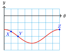
86. \(f(\theta) = 1 + \sin \theta\)

    

Applications

87. The tide in Yorktown is approximated by the function\[h(t)=1.4-1.4 \cos (0.51 t)\nonumber \]measured in feet above low tide, where \(t\) is the number of hours since the last low tide.

    1. What are the midline, period, and amplitude?

    2. Graph \(h(t)\) for two periods, labeling the points that correspond to high tide and low tide.

    3. If the last low tide occurred at 5:00 am, predict when the next high and low tides will occur.

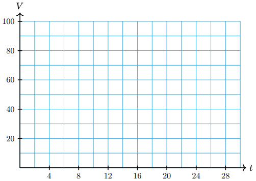
88. When observed from Earth, the moon looks like a disk that is partially visible and partially in shadow. The percentage of the disk that is visible can be approximated by\[V(t)=50 \cos (0.21 t)+50\nonumber \]where \(t\) is the number of days since the last full moon.

    1. Graph \(V(t)\) in the window\[X_{\text{min}} = 0, X_{\text{max}} = 30\nonumber \]\[Y_{\text{min}} = 0, Y_{\text{max}} = 120\nonumber \]

       

    2. Sketch the graph on the grid.

    3. Label on your graph the points that correspond to full moon, half moon, and new moon. (New moon occurs when the part of the moon receiving sunlight is facing directly away from the Earth.)

    4. At what times during the lunar month is \(25 \%\) of the moon visible? Mark those points on your graph.

    5. During which days is less than \(50 \%\) of the moon visible? Mark the corresponding points on your graph.

89. The tide in Malibu is approximated by the function\[h(t)=2.5-2.5 \cos (0.5 t)\nonumber \]measured in feet above low tide, where \(t\) is the number of hours since the last low tide.

    1. Graph \(h(t)\) in the window\[X_{\text{min}} = 0, X_{\text{max}} = 25\nonumber \]\[Y_{\text{min}} = 0, Y_{\text{max}} = 6\nonumber \]

       

    2. Sketch the graph on the grid.

    3. Label on your graph the points that correspond to high tide and low tide.

    4. How high is high tide, and at what times does it occur?

    5. At what times during the 25-hour period is the tide 4 feet above low tide? Mark those points on your graph.

    6. Kathie walks along the beach only when the tide is below 1 foot. Find the intervals on your graph when the tide is below 1 foot.

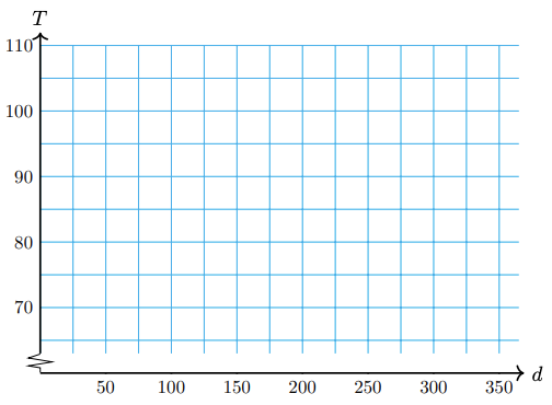
90. The average daily high temperature in the town of Beardsley, Arizona is approximated by the function\[T(d)=85.5-19.5 \cos (0.0175 d-0.436)\nonumber \]where the temperature is measured in degrees Fahrenheit, and \(d\) is the number of days since January 1.

    1. Graph \(T(d)\) in the window\[X_{\text{min}} = 0, X_{\text{max}} = 365\nonumber \]\[Y_{\text{min}} = 0, Y_{\text{max}} = 110\nonumber \]

       

    2. Sketch the graph on the grid.

    3. Label on your graph the points that correspond to highest and lowest average temperature.

    4. What is the hottest day and what is its average temperature? What is the day with the lowest average temperature, and what is that temperature?

    5. At what times during the year are average high temperatures above \(90^{\circ}\)? Mark those points on your graph.

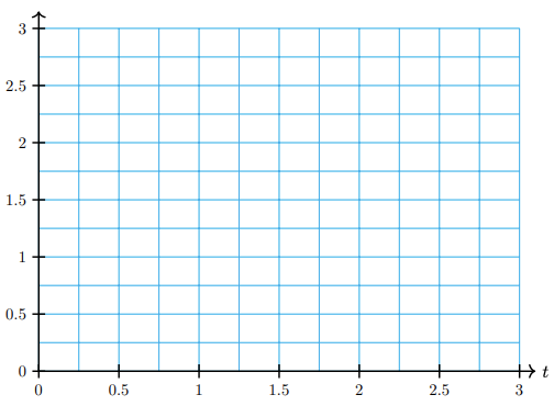
91. A weight is suspended from the ceiling on a spring. The weight is pushed straight up, compressing the spring, then released. The height of the weight above the ground is given by the function\[H(t)=2+0.5 \cos (6 t)\nonumber \]where the height is measured in meters, and \(t\) is the number of seconds since the mass was released.

    1. Graph \(H(t)\) in the window\[X_{\text{min}} = 0, X_{\text{max}} = 3\nonumber \]\[Y_{\text{min}} = 0, Y_{\text{max}} = 3\nonumber \]

       

    2. Sketch the graph on the grid.

    3. Label on your graph the points that correspond to highest and lowest positions of the mass.

    4. How high is highest point, and when is that height attained during the first 3 seconds?

    5. How high is lowest point, and when is that height attained during the first 3 seconds?

    6. Find the intervals during the first 3 seconds when the mass is less than 2 meters above the ground.

For Problems 92 - #, write an equation for the sinusoidal function whose graph is shown.

92. The number of hours of daylight in Salt Lake City varies from a minimum of 9.6 hours on the winter solstice to a maximum of 14.4 hours on the summer solstice. Time is measured in months, starting at the winter solstice.

    

93. A weight is 6.5 feet above the floor, suspended from the ceiling by a spring. The weight is pulled down to 5 feet above the floor and released, rising past 6.5 feet in 0.5 seconds before attaining its maximum height of feet. The weight oscillates between its minimum and maximum height.

    

94. Although the moon is spherical, what we see from Earth looks like a disk, sometimes only partly visible. The percentage of the moon’s disk that is visible varies between 0 (at new moon) to 100 (at full moon), over a 28-day cycle.