Chapter 13: Non-Right Triangle Trigonometry

Last updated
Save as PDF

Page ID: 173866

Roy Simpson & Katherine Yoshiwara
Los Angeles Pierce College

$ \newcommand{\vecs}[1]{\overset { \scriptstyle \rightharpoonup} {\mathbf{#1}} } $

$ \newcommand{\vecd}[1]{\overset{-\!-\!\rightharpoonup}{\vphantom{a}\smash {#1}}} $

$ \newcommand{\id}{\mathrm{id}}$ $ \newcommand{\Span}{\mathrm{span}}$

( \newcommand{\kernel}{\mathrm{null}\,}\) $ \newcommand{\range}{\mathrm{range}\,}$

$ \newcommand{\RealPart}{\mathrm{Re}}$ $ \newcommand{\ImaginaryPart}{\mathrm{Im}}$

$ \newcommand{\Argument}{\mathrm{Arg}}$ $ \newcommand{\norm}[1]{\| #1 \|}$

$ \newcommand{\inner}[2]{\langle #1, #2 \rangle}$

$ \newcommand{\Span}{\mathrm{span}}$

$ \newcommand{\id}{\mathrm{id}}$

$ \newcommand{\Span}{\mathrm{span}}$

$ \newcommand{\kernel}{\mathrm{null}\,}$

$ \newcommand{\range}{\mathrm{range}\,}$

$ \newcommand{\RealPart}{\mathrm{Re}}$

$ \newcommand{\ImaginaryPart}{\mathrm{Im}}$

$ \newcommand{\Argument}{\mathrm{Arg}}$

$ \newcommand{\norm}[1]{\| #1 \|}$

$ \newcommand{\inner}[2]{\langle #1, #2 \rangle}$

$ \newcommand{\Span}{\mathrm{span}}$ $ \newcommand{\AA}{\unicode[.8,0]{x212B}}$

$ \newcommand{\vectorA}[1]{\vec{#1}} % arrow$

$ \newcommand{\vectorAt}[1]{\vec{\text{#1}}} % arrow$

$ \newcommand{\vectorB}[1]{\overset { \scriptstyle \rightharpoonup} {\mathbf{#1}} } $

$ \newcommand{\vectorC}[1]{\textbf{#1}} $

$ \newcommand{\vectorD}[1]{\overrightarrow{#1}} $

$ \newcommand{\vectorDt}[1]{\overrightarrow{\text{#1}}} $

$ \newcommand{\vectE}[1]{\overset{-\!-\!\rightharpoonup}{\vphantom{a}\smash{\mathbf {#1}}}} $

$ \newcommand{\vecs}[1]{\overset { \scriptstyle \rightharpoonup} {\mathbf{#1}} } $

$ \newcommand{\vecd}[1]{\overset{-\!-\!\rightharpoonup}{\vphantom{a}\smash {#1}}} $

$\newcommand{\avec}{\mathbf a}$ $\newcommand{\bvec}{\mathbf b}$ $\newcommand{\cvec}{\mathbf c}$ $\newcommand{\dvec}{\mathbf d}$ $\newcommand{\dtil}{\widetilde{\mathbf d}}$ $\newcommand{\evec}{\mathbf e}$ $\newcommand{\fvec}{\mathbf f}$ $\newcommand{\nvec}{\mathbf n}$ $\newcommand{\pvec}{\mathbf p}$ $\newcommand{\qvec}{\mathbf q}$ $\newcommand{\svec}{\mathbf s}$ $\newcommand{\tvec}{\mathbf t}$ $\newcommand{\uvec}{\mathbf u}$ $\newcommand{\vvec}{\mathbf v}$ $\newcommand{\wvec}{\mathbf w}$ $\newcommand{\xvec}{\mathbf x}$ $\newcommand{\yvec}{\mathbf y}$ $\newcommand{\zvec}{\mathbf z}$ $\newcommand{\rvec}{\mathbf r}$ $\newcommand{\mvec}{\mathbf m}$ $\newcommand{\zerovec}{\mathbf 0}$ $\newcommand{\onevec}{\mathbf 1}$ $\newcommand{\real}{\mathbb R}$ $\newcommand{\twovec}[2]{\left[\begin{array}{r}#1 \\ #2 \end{array}\right]}$ $\newcommand{\ctwovec}[2]{\left[\begin{array}{c}#1 \\ #2 \end{array}\right]}$ $\newcommand{\threevec}[3]{\left[\begin{array}{r}#1 \\ #2 \\ #3 \end{array}\right]}$ $\newcommand{\cthreevec}[3]{\left[\begin{array}{c}#1 \\ #2 \\ #3 \end{array}\right]}$ $\newcommand{\fourvec}[4]{\left[\begin{array}{r}#1 \\ #2 \\ #3 \\ #4 \end{array}\right]}$ $\newcommand{\cfourvec}[4]{\left[\begin{array}{c}#1 \\ #2 \\ #3 \\ #4 \end{array}\right]}$ $\newcommand{\fivevec}[5]{\left[\begin{array}{r}#1 \\ #2 \\ #3 \\ #4 \\ #5 \\ \end{array}\right]}$ $\newcommand{\cfivevec}[5]{\left[\begin{array}{c}#1 \\ #2 \\ #3 \\ #4 \\ #5 \\ \end{array}\right]}$ $\newcommand{\mattwo}[4]{\left[\begin{array}{rr}#1 \amp #2 \\ #3 \amp #4 \\ \end{array}\right]}$ $\newcommand{\laspan}[1]{\text{Span}\{#1\}}$ $\newcommand{\bcal}{\cal B}$ $\newcommand{\ccal}{\cal C}$ $\newcommand{\scal}{\cal S}$ $\newcommand{\wcal}{\cal W}$ $\newcommand{\ecal}{\cal E}$ $\newcommand{\coords}[2]{\left\{#1\right\}_{#2}}$ $\newcommand{\gray}[1]{\color{gray}{#1}}$ $\newcommand{\lgray}[1]{\color{lightgray}{#1}}$ $\newcommand{\rank}{\operatorname{rank}}$ $\newcommand{\row}{\text{Row}}$ $\newcommand{\col}{\text{Col}}$ $\renewcommand{\row}{\text{Row}}$ $\newcommand{\nul}{\text{Nul}}$ $\newcommand{\var}{\text{Var}}$ $\newcommand{\corr}{\text{corr}}$ $\newcommand{\len}[1]{\left|#1\right|}$ $\newcommand{\bbar}{\overline{\bvec}}$ $\newcommand{\bhat}{\widehat{\bvec}}$ $\newcommand{\bperp}{\bvec^\perp}$ $\newcommand{\xhat}{\widehat{\xvec}}$ $\newcommand{\vhat}{\widehat{\vvec}}$ $\newcommand{\uhat}{\widehat{\uvec}}$ $\newcommand{\what}{\widehat{\wvec}}$ $\newcommand{\Sighat}{\widehat{\Sigma}}$ $\newcommand{\lt}{<}$ $\newcommand{\gt}{>}$ $\newcommand{\amp}{&}$ $\definecolor{fillinmathshade}{gray}{0.9}$

$Screen Shot 2022-09-27 at 10.37.42 AM.png$

The first science developed by humans is probably Astronomy. Before the invention of clocks and calendars, early people looked to the night sky to help them keep track of time. What is the best time to plant crops, and when will they ripen? On what day exactly do important religious festivals fall?

By tracking the motions of the stars, early astronomers could identify the summer and winter solstices and the equinoxes. The rising and setting of certain stars marked the hours of the night.

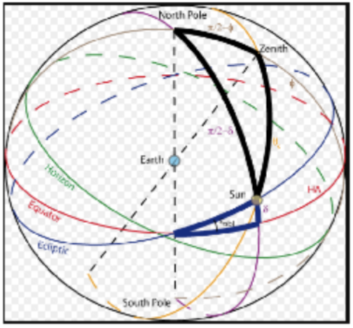
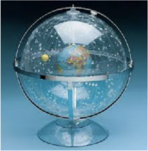
If we think of the stars as traveling on a dome above the Earth, we create the celestial sphere. Actually, of course, the Earth itself rotates among the stars, but for calculating the motions of heavenly objects, this model works very well.

$Screen Shot 2022-09-27 at 10.38.18 AM.png$

Babylonian astronomers kept detailed records on the motion of the planets, and were able to predict solar and lunar eclipses. All of this required familiarity with angular distances measured on the celestial sphere.

To find angles and distances on this imaginary sphere, astronomers invented techniques that are now part of spherical trigonometry. The laws of sines and cosines were first stated in this context, in a slightly different form than the laws for plane trigonometry.

$Screen Shot 2022-09-27 at 10.39.34 AM.png$

On a sphere, a great-circle lies in a plane passing through the sphere’s center. It gives the shortest distance between any two points on a sphere, and is the analogue of a straight line on a plane. A spherical angle is formed where two such arcs intersect, and a spherical triangle is made up of three arcs of great circles.

The spherical law of sines was first introduced in Europe in 1464 by Johann Muller, also known as Regiomontus, who wrote:

"You, who wish to study great and wondrous things, who wonder about the movement of the stars, must read these theorems about triangles. ... For no one can bypass the science of triangles and reach a satisfying knowledge of the stars.”

13.1: The Law of Sines
This section covers the Law of Sines, including its derivation, and how to use it to find missing sides and angles in oblique triangles. It includes examples, practical applications, and solving triangles, addressing the ambiguous case and its implications. The section emphasizes step-by-step solutions and advises on efficient calculation techniques to minimize errors.
13.2: The Law of Cosines
This section discusses the Law of Cosines, including its derivation, and how to apply it to find missing sides and angles in any triangle. It covers practical examples and applications such as solving navigation problems. The Law of Cosines is presented as a generalization of the Pythagorean Theorem, useful for triangles that are not right-angled. The section also emphasizes the importance of following the order of operations and choosing angles wisely when applying the law.
13.3: Areas
This section explains how to find the area of a triangle using trigonometric methods. It covers two such formulas - one for triangles with two known sides and the included angle, and the other (Heron's Formula) for when all three sides are known. Practical examples and exercises illustrate the application of these formulas.
13.4: Vectors - A Geometric Approach
This section introduces vectors from a geometric perspective, covering definitions, notation, and operations. It explains position vectors, scalar multiplication, vector addition, and the concepts of displacement and resultant vectors. The section also addresses vector components, their magnitudes, and applications in velocity and other contexts. Detailed examples and exercises help illustrate these concepts, providing a comprehensive understanding of vectors in geometric terms.
13.5: Vectors - An Algebraic Approach
This section covers vectors from an algebraic perspective, including expressing vectors in coordinate form, converting between geometric and coordinate forms, and performing vector operations such as scalar multiplication and addition. It introduces unit vectors, discusses their significance, and explores their use in practical applications like force and equilibrium problems. The section includes examples and exercises to reinforce understanding of algebraic vector manipulation.

Search

Text Color

Text Size

Margin Size

Font Type