
5.7: A.7- Tangent Lines and Velocity
- Page ID
- 116545

\( \newcommand{\vecs}[1]{\overset { \scriptstyle \rightharpoonup} {\mathbf{#1}} } \)
\( \newcommand{\vecd}[1]{\overset{-\!-\!\rightharpoonup}{\vphantom{a}\smash {#1}}} \)
\( \newcommand{\dsum}{\displaystyle\sum\limits} \)
\( \newcommand{\dint}{\displaystyle\int\limits} \)
\( \newcommand{\dlim}{\displaystyle\lim\limits} \)
\( \newcommand{\id}{\mathrm{id}}\) \( \newcommand{\Span}{\mathrm{span}}\)
( \newcommand{\kernel}{\mathrm{null}\,}\) \( \newcommand{\range}{\mathrm{range}\,}\)
\( \newcommand{\RealPart}{\mathrm{Re}}\) \( \newcommand{\ImaginaryPart}{\mathrm{Im}}\)
\( \newcommand{\Argument}{\mathrm{Arg}}\) \( \newcommand{\norm}[1]{\| #1 \|}\)
\( \newcommand{\inner}[2]{\langle #1, #2 \rangle}\)
\( \newcommand{\Span}{\mathrm{span}}\)
\( \newcommand{\id}{\mathrm{id}}\)
\( \newcommand{\Span}{\mathrm{span}}\)
\( \newcommand{\kernel}{\mathrm{null}\,}\)
\( \newcommand{\range}{\mathrm{range}\,}\)
\( \newcommand{\RealPart}{\mathrm{Re}}\)
\( \newcommand{\ImaginaryPart}{\mathrm{Im}}\)
\( \newcommand{\Argument}{\mathrm{Arg}}\)
\( \newcommand{\norm}[1]{\| #1 \|}\)
\( \newcommand{\inner}[2]{\langle #1, #2 \rangle}\)
\( \newcommand{\Span}{\mathrm{span}}\) \( \newcommand{\AA}{\unicode[.8,0]{x212B}}\)
\( \newcommand{\vectorA}[1]{\vec{#1}} % arrow\)
\( \newcommand{\vectorAt}[1]{\vec{\text{#1}}} % arrow\)
\( \newcommand{\vectorB}[1]{\overset { \scriptstyle \rightharpoonup} {\mathbf{#1}} } \)
\( \newcommand{\vectorC}[1]{\textbf{#1}} \)
\( \newcommand{\vectorD}[1]{\overrightarrow{#1}} \)
\( \newcommand{\vectorDt}[1]{\overrightarrow{\text{#1}}} \)
\( \newcommand{\vectE}[1]{\overset{-\!-\!\rightharpoonup}{\vphantom{a}\smash{\mathbf {#1}}}} \)
\( \newcommand{\vecs}[1]{\overset { \scriptstyle \rightharpoonup} {\mathbf{#1}} } \)
\(\newcommand{\longvect}{\overrightarrow}\)
\( \newcommand{\vecd}[1]{\overset{-\!-\!\rightharpoonup}{\vphantom{a}\smash {#1}}} \)
\(\newcommand{\avec}{\mathbf a}\) \(\newcommand{\bvec}{\mathbf b}\) \(\newcommand{\cvec}{\mathbf c}\) \(\newcommand{\dvec}{\mathbf d}\) \(\newcommand{\dtil}{\widetilde{\mathbf d}}\) \(\newcommand{\evec}{\mathbf e}\) \(\newcommand{\fvec}{\mathbf f}\) \(\newcommand{\nvec}{\mathbf n}\) \(\newcommand{\pvec}{\mathbf p}\) \(\newcommand{\qvec}{\mathbf q}\) \(\newcommand{\svec}{\mathbf s}\) \(\newcommand{\tvec}{\mathbf t}\) \(\newcommand{\uvec}{\mathbf u}\) \(\newcommand{\vvec}{\mathbf v}\) \(\newcommand{\wvec}{\mathbf w}\) \(\newcommand{\xvec}{\mathbf x}\) \(\newcommand{\yvec}{\mathbf y}\) \(\newcommand{\zvec}{\mathbf z}\) \(\newcommand{\rvec}{\mathbf r}\) \(\newcommand{\mvec}{\mathbf m}\) \(\newcommand{\zerovec}{\mathbf 0}\) \(\newcommand{\onevec}{\mathbf 1}\) \(\newcommand{\real}{\mathbb R}\) \(\newcommand{\twovec}[2]{\left[\begin{array}{r}#1 \\ #2 \end{array}\right]}\) \(\newcommand{\ctwovec}[2]{\left[\begin{array}{c}#1 \\ #2 \end{array}\right]}\) \(\newcommand{\threevec}[3]{\left[\begin{array}{r}#1 \\ #2 \\ #3 \end{array}\right]}\) \(\newcommand{\cthreevec}[3]{\left[\begin{array}{c}#1 \\ #2 \\ #3 \end{array}\right]}\) \(\newcommand{\fourvec}[4]{\left[\begin{array}{r}#1 \\ #2 \\ #3 \\ #4 \end{array}\right]}\) \(\newcommand{\cfourvec}[4]{\left[\begin{array}{c}#1 \\ #2 \\ #3 \\ #4 \end{array}\right]}\) \(\newcommand{\fivevec}[5]{\left[\begin{array}{r}#1 \\ #2 \\ #3 \\ #4 \\ #5 \\ \end{array}\right]}\) \(\newcommand{\cfivevec}[5]{\left[\begin{array}{c}#1 \\ #2 \\ #3 \\ #4 \\ #5 \\ \end{array}\right]}\) \(\newcommand{\mattwo}[4]{\left[\begin{array}{rr}#1 \amp #2 \\ #3 \amp #4 \\ \end{array}\right]}\) \(\newcommand{\laspan}[1]{\text{Span}\{#1\}}\) \(\newcommand{\bcal}{\cal B}\) \(\newcommand{\ccal}{\cal C}\) \(\newcommand{\scal}{\cal S}\) \(\newcommand{\wcal}{\cal W}\) \(\newcommand{\ecal}{\cal E}\) \(\newcommand{\coords}[2]{\left\{#1\right\}_{#2}}\) \(\newcommand{\gray}[1]{\color{gray}{#1}}\) \(\newcommand{\lgray}[1]{\color{lightgray}{#1}}\) \(\newcommand{\rank}{\operatorname{rank}}\) \(\newcommand{\row}{\text{Row}}\) \(\newcommand{\col}{\text{Col}}\) \(\renewcommand{\row}{\text{Row}}\) \(\newcommand{\nul}{\text{Nul}}\) \(\newcommand{\var}{\text{Var}}\) \(\newcommand{\corr}{\text{corr}}\) \(\newcommand{\len}[1]{\left|#1\right|}\) \(\newcommand{\bbar}{\overline{\bvec}}\) \(\newcommand{\bhat}{\widehat{\bvec}}\) \(\newcommand{\bperp}{\bvec^\perp}\) \(\newcommand{\xhat}{\widehat{\xvec}}\) \(\newcommand{\vhat}{\widehat{\vvec}}\) \(\newcommand{\uhat}{\widehat{\uvec}}\) \(\newcommand{\what}{\widehat{\wvec}}\) \(\newcommand{\Sighat}{\widehat{\Sigma}}\) \(\newcommand{\lt}{<}\) \(\newcommand{\gt}{>}\) \(\newcommand{\amp}{&}\) \(\definecolor{fillinmathshade}{gray}{0.9}\)- Absolute Prerequisites
-
- Algebra
- Functions
- Evaluating at a constant
- Linear Functions
- Equation of a line
- Slope
- Rate of Change
- Functions
- Algebra
- Relate the rate of change of a function to the slope of a secant line.
- Describe the concept and process of approximating the tangent line to a function at a given point.
- Recognize a tangent to a curve at a point as the limit of secant lines.
- Identify instantaneous velocity as the limit of average velocity over a small time interval.
- Distinguish when technology is appropriate to use within a given problem.
As we embark on our study of Calculus, we shall see how its development arose from common solutions to practical problems in areas such as engineering physics. Two key problems led to the initial formulation of calculus: (1) the tangent problem, or how to determine the slope of a line tangent to a curve at a point; and (2) the area problem, or how to determine the area under a curve. Chapters two through four focus on the first of these problems. We will approach the area problem at the end of this course.
Rates of Change
Rate of change is one of the most critical concepts in Calculus. We begin our investigation of rates of change by looking at the graphs of the three lines \(f(x)=−2x−3,\; g(x)=\dfrac{1}{2}x+1\), and \(h(x)=2\), shown in Figure \(\PageIndex{1}\).
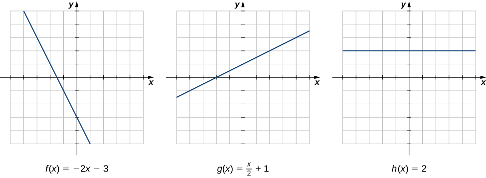
Figure \(\PageIndex{1}\): The rate of change of a linear function is constant in each of these three graphs, with the constant determined by the slope.
As we move from left to right along the graph of \(f(x)=−2x−3\), we see that the graph decreases at a constant rate. For every \(1\) unit we move to the right along the \(x\)-axis, the \(y\)-coordinate decreases by \(2\) units. This rate of change is determined by the slope (\(−2\)) of the line. Similarly, the slope of \(1/2\) in the function \(g(x)\) tells us that for every change in \(x\) of \(1\) unit there is a corresponding change in \(y\) of \(1/2\) unit. The function \(h(x)=2\) has a slope of zero, indicating that the values of the function remain constant. We see that the slope of each linear function indicates the rate of change of the function.
The rate of change at any given point, \((a, f(a))\), of a linear function is constant and equal to the slope of the function.
Compare the graphs of these three functions with the graph of \(k(x)=x^2\) (Figure \(\PageIndex{2}\)). The graph of \(k(x)=x^2\) starts from the left by decreasing rapidly, then begins to decrease more slowly and level off, and then finally begins to increase - slowly at first, followed by an increasing rate of increase as it moves toward the right. Unlike a linear function, no single number represents the rate of change for this function. We quite naturally ask: How do we measure the rate of change of a nonlinear function? Since the rate of change for a nonlinear function is ever-changing, is it possible to determine the rate of change at a specific point?

Figure \(\PageIndex{2}\): The function \(k(x)=x^2\) does not have a constant rate of change.
Before we go any further, a word of caution is needed.
Lines have slopes; however, nonlinear curves do not. That is, it's incorrect to talk about the "slope" of the nonlinear function \(k(x) = x^2\).
How do we overcome this restriction in language? When referencing the "steepness" of a nonlinear function at a point \((a, f(a))\), we instead refer to the slope of the tangent line at this point.
In geometry, the tangent line (or simply tangent) to a plane curve at a given point is the straight line that "just touches" the curve at that point.1 As it passes through the point where the tangent line and the curve meet, called the point of tangency, the tangent line is "going in the same direction" as the curve, and is thus the best straight-line approximation to the curve at that point.
Therefore, if you wanted to tell someone how steep the function \(k(x) = x^2\) is at the point \((a, f(a))\), you would reference the slope of the tangent line to the function at that point. Another phrase used for the slope of the tangent line is the instantaneous rate of change of \(f(x)\) at \((a,f(a))\).
The blue line that intersects \(k(x) = x^2\) locally at the purple point is called the tangent line to the curve \(k(x)\) at \((a, k(a))\).
The graph of \(k(x) = x^2\) and the tangent line to \(k(x)\) at \((a, k(a))\).
Interact: Move the point.
Observation: The slope of the tangent line changes. For example, if you move the point to \((1/2,1/4)\), you will see that the slope of the tangent line is \(1\). Therefore, the instantaneous rate of change of \(k(x) = x^2\) at \((1/2, 1/4)\) is \(1\).
Tangent and Secant Lines
We can approximate the instantaneous rate of change of a function \(f(x)\) at a point \((a,f(a))\) on its graph by taking another point \((x,f(x))\) on the graph of \(f(x)\), drawing a line through the two points, and calculating the slope of the resulting line. Such a line is called a secant line. Figure \(\PageIndex{3}\) shows a secant line to a function \(f(x)\) at a point \((a,f(a))\).

Figure \(\PageIndex{3}\): The slope of a secant line through a point \((a,f(a))\) estimates the instantaneous rate of change of the function at the point \((a,f(a))\).
We formally define a secant line as follows:
The secant line (also known simply as the secant) to the function \(f(x)\) through the points \((a,f(a))\) and \((x,f(x))\) is the line passing through these points. Its slope is given by\[m_{sec}=\dfrac{f(x)−f(a)}{x−a}. \label{secantslope} \]
The accuracy of approximating the instantaneous rate of change of the function with a secant line depends on how close \(x\) is to \(a\). As we see in Figure \(\PageIndex{4}\), if \(x\) is closer to \(a\), the slope of the secant line looks to be a better measure of the instantaneous rate of change of \(f(x)\) at \(a\). There are times when dragging \((x,f(x))\) closer to \((a,f(a))\) will not provide a better estimate of the tangent line, but we will avoid those instances for now.

Figure \(\PageIndex{4}\): As \(x\) gets closer to \(a\), the slope of the secant line becomes a better approximation to the rate of change of the function \(f(x)\) at \(a\).
The secant lines themselves approach the tangent line to the function \(f(x)\) at \(a\) (Figure \(\PageIndex{5}\)). As stated previously, the slope of the tangent line to the graph at \(a\) is a measure of the instantaneous rate of change of the function at \(a\). This value is incredibly important in Calculus.

Figure \(\PageIndex{5}\): Solving the Tangent Problem: As \(x\) approaches \(a\), the secant lines approach the tangent line.
This entire section is focused on using the slopes of the secant lines to approximate the slope of the tangent line to \(f(x)\) at \((a,f(a))\). The point \((a,f(a))\) is commonly referred to as the anchor point because it is "anchored" to a single spot while the secondary point, \((x,f(x))\), is moved toward it. In Figures \(\PageIndex{4}\) and \(\PageIndex{5}\), you can see the secant lines each include the anchor point \((a,f(a))\).
Use this Interactive Element to help you understand the difference between secant lines, the tangent line, rates of change, and the instantaneous rate of change of a function at a point.
Interact: Move the point \(P\) close to the anchor point. You can also move the anchor point elsewhere.
Observation: As \(P\) gets closer to the anchor point, the slope of the secant line begins to approximate the slope of the tangent line at the anchor point.
Question: What happens when the two points meet? Why do you think this happens?
Approximating the Slope of the Tangent Line
The next example illustrates how to find slopes of secant lines. These slopes estimate the slope of the tangent line or, equivalently, the instantaneous rate of change of the function at the point at which the slopes are calculated.
Estimate the instantaneous rate of change (slope of the tangent line) to \(f(x)=x^2\) at \(x=1\) by finding slopes of secant lines through \((1,1)\) and each of the following points on the graph of \(f(x)=x^2\).
- \((2,4)\)
- \(\left(\frac{3}{2},\frac{9}{4}\right)\)
- Solutions
-
Use the formula for the slope of a secant line (Equation \ref{secantslope}).
- \(m_{sec}=\frac{4−1}{2−1}=3\)
- \(m_{sec}=\frac{\frac{9}{4}−1}{\frac{3}{2}−1}=\frac{5}{2}=2.5\)
The point in part b. is closer to the point \((1,1)\), so the slope of \(2.5\) is closer to the slope of the tangent line. A good estimate for the slope of the tangent would be in the range of \(2\) to \(2.5\) (Figure \(\PageIndex{6}\)).

The secant lines to \(f(x)=x^2\) at \((1,1)\) through (a) \((2,4)\) and (b) \(\left(\frac{3}{2},\frac{9}{4}\right)\) provide successively closer approximations to the tangent line to \(f(x)=x^2\) at \((1,1)\).
Estimate the slope of the tangent line (instantaneous rate of change) to \(f(x)=x^2\) at \(x=1\) by finding slopes of secant lines through \((1,1)\) and the point \(\left(\frac{5}{4},\frac{25}{16}\right)\) on the graph of \(f(x)=x^2\).
- Answer
-
\(2.25\)
Estimate the slope of the tangent line to the function \(g(x) = -2 \sin{(\pi x)} + 2\) at \(x = \frac{1}{4}\) to three decimal places.
- Solution
-
In this example, we are not given an explicit list of points to try. Instead, there is an implicit assumption that we will create our own list of \(x\)-values approaching \(\frac{1}{4}\). It is important to include \(x\)-values both greater than and less than \(\frac{1}{4}\) in our trials. I will demonstrate two different approaches both of which should be read for understanding.
In either approach, we will need to use the formula for the slope of the secant line (Equation \ref{secantslope}); however, the implementation of the formula will differ between methods. Before going into the methods, we need to compute \(g\left(\frac{1}{4}\right)\).\[ \begin{array}{rcl}
g\left( \dfrac{1}{4} \right) & = & -2 \sin{\left(\dfrac{\pi}{4}\right)} + 2 \\[16pt]
& = & -\dfrac{2}{\sqrt{2}} + 2 \\[16pt]
& = & -\sqrt{2} + 2 \\[16pt]
& = & 2 - \sqrt{2} \\
\end{array} \nonumber \]Method #1: Explicitly Choosing Values Near \(1/4 = 0.25\)
The first approach is the one most students will start with because it mimics how they learned slope. We successively pick numbers closer and closer to \(0.25\) (from the right and left of \(0.25\) on the number line) to get an approximation to the slope of the tangent line.
Prior to "plugging in" values near \(0.25\), we write the secant slope formula, substitute any values we have been given (or have computed), and then simplify.\[ \begin{array}{rcl}
m_{sec} & = & \dfrac{g(x) - g(a)}{x - a} \\[16pt]
& = & \dfrac{-2 \sin{(\pi x)} + 2 - g\left(\frac{1}{4}\right)}{x - \frac{1}{4}} \\[16pt]
& = & \dfrac{-2 \sin{(\pi x)} + 2 - \left(2 - \sqrt{2} \right)}{x - \frac{1}{4}} \\[16pt]
& = & \dfrac{-2 \sin{(\pi x)} + 2 - 2 + \sqrt{2} }{x - \frac{1}{4}} \\[16pt]
& = & \dfrac{-2 \sin{(\pi x)} + \sqrt{2} }{x - \frac{1}{4}} \\[16pt]
& = & \dfrac{-8 \sin{(\pi x)} + 4 \sqrt{2} }{4 x - 1} \\
\end{array} \nonumber \]Being able to do the algebraic "pre-work" for a problem is critical to success in Calculus. If you were lost on any of the manipulations above, it is best to review Chapter 1 of this text, or review your College Algebra textbook.
At this point, we are ready to substitute values for \(x\) that approach \(0.25\). The following table contains values approaching \(0.25\) from the right (on the number line).
\(x\) \(m_{sec} = \frac{-8 \sin{(\pi x)} + 4 \sqrt{2} }{4 x - 1}\) 0.35 \(\approx -3.6779949 \) 0.26 \(\approx -4.3723692 \) 0.251 \(\approx -4.4358968 \) 0.2501 \(\approx -4.442185 \) 0.25001 \(\approx -4.4428131 \) 0.250001 \(\approx -4.442876 \) The next table shows similar computations for values of \(x\) approaching \(0.25\) from the left (on the number line).
\(x\) \(m_{sec} = \frac{-8 \sin{(\pi x)} + 4 \sqrt{2} }{4 x - 1}\) 0.15 \(\approx -5.0623256 \) 0.24 \(\approx -4.5119351 \) 0.249 \(\approx -4.4498545 \) 0.2499 \(\approx -4.4435808 \) 0.24999 \(\approx -4.4429527 \) 0.249999 \(\approx -4.4428899 \) In both cases, it looks like the slopes of the secant lines are approaching roughly \(-4.443\) (when rounded to the third decimal place).
Are your values not matching those in the table?
Remember, Calculus requires angles in radians. From this point forward, whenever you are working on a problem involving trigonometric functions and you require a calculator, be sure to set the calculator to radian mode!
Method #2: Choosing "Wiggles"
The second approach is the preferred approach for the rest of Calculus. We successively pick smaller and smaller numbers to decrease the "wiggled distance" between \(a\) and \(x\).
The "pre-work" is slightly different than what we did previously. Instead working with \(x\), we let \(x = a + h\) and allow \(h\) to get smaller and smaller. The lower the value of \(h\), the closer \(x = a + h\) is to \(a\). Like before, prior to "plugging in" smaller and smaller values of \(h\), we write the secant slope formula, substitute any values we have been given (or have computed), and then simplify.\[ \begin{array}{rcl}
m_{sec} & = & \dfrac{g(x) - g(a)}{x - a} \\[16pt]
& = & \dfrac{g(a + h) - g(a)}{a + h - a} \\[16pt]
& = & \dfrac{g(a + h) - g(a)}{h} \\[16pt]
& = & \dfrac{g(0.25 + h) - g(0.25)}{h} \\[16pt]
& = & \dfrac{-2 \sin{\left(\pi (0.25 + h)\right)} + 2 - g(0.25)}{h} \\[16pt]
& = & \dfrac{-2 \sin{\left(\pi (0.25 + h)\right)} + 2 - \left(2 - \sqrt{2} \right)}{h} \\[16pt]
& = & \dfrac{-2 \sin{\left(\pi (0.25 + h)\right)} + 2 - 2 + \sqrt{2} }{h} \\[16pt]
& = & \dfrac{-2 \sin{\left(\pi (0.25 + h)\right)} + \sqrt{2} }{h} \\
\end{array} \nonumber \]At this point, we are ready to substitute values for \(h\) that approach \(0\). The following table contains values approaching \(0\) from the right (on the number line).
\(h\) \(m_{sec} = \frac{-2 \sin{\left(\pi (0.25 + h)\right)} + \sqrt{2} }{h}\) 0.1 \(\approx -3.6779949 \) 0.01 \(\approx -4.3723692 \) 0.001 \(\approx -4.4358968 \) 0.0001 \(\approx -4.442185 \) 0.00001 \(\approx -4.4428131 \) 0.000001 \(\approx -4.442876 \) The next table shows similar computations for values of \(x\) approaching \(0\) from the left (on the number line).
\(h\) \(m_{sec} = \frac{-2 \sin{\left(\pi (0.25 + h)\right)} + \sqrt{2} }{h}\) -0.1 \(\approx -5.0623256 \) -0.01 \(\approx -4.5119351 \) -0.001 \(\approx -4.4498545 \) -0.0001 \(\approx -4.4435808 \) -0.00001 \(\approx -4.4429527 \) -0.000001 \(\approx -4.4428899 \) In both cases, it looks like the slopes of the secant lines are approaching roughly \(-4.443\) (when rounded to the third decimal place).
Result
In the end, both methods produce the same results, however, the second method demonstrates a significant building block for the study of Calculus. While the "pre-work" was slightly more involved, the inputs (the values that were being substituted in for \(h\)) not only were easier to work with, but conceptually made sense. We are just decreasing the "space" between the anchor point and \((x, f(x))\) to something near zero.
Instantaneous Velocity
We continue our investigation by exploring a related question. Keeping in mind that velocity may be thought of as the rate of change of position, suppose that we have a function, \(s(t)\), that gives the position of an object along a coordinate axis at any given time \(t\). Can we use these same ideas to create a reasonable definition of the instantaneous velocity at a given time \(t=a?\) We start by approximating the instantaneous velocity with an average velocity. First, recall that the speed of an object traveling at a constant rate is the ratio of the distance traveled to the length of time it has traveled. We define the average velocity of an object over a time period to be the change in its position divided by the length of the time period.
Let \(s(t)\) be the position of an object moving along a coordinate axis at time \(t\). The average velocity of the object over a time interval \([a,t]\) where \(a<t\) (or \([t,a]\) if \(t<a)\) is\[v_{avg}=\dfrac{s(t)−s(a)}{t−a}. \label{avgvel} \]
As \(t\) is chosen closer to \(a\), the average velocity becomes closer to the instantaneous velocity. Note that finding the average velocity of a position function over a time interval is essentially the same as finding the slope of a secant line to a function. Furthermore, to find the slope of a tangent line at a point \(a\), we let the \(x\)-values approach \(a\) in the slope of the secant line. Similarly, to find the instantaneous velocity at time \(a\), we let the \(t\)-values approach \(a\) in the average velocity. This process of letting \(x\) or \(t\) approach \(a\) in an expression is called taking a limit. Thus, we may define the instantaneous velocity as follows.
For a position function \(s(t)\), the instantaneous velocity at a time \(t=a\) is the value that the average velocities approach on intervals of the form \([a,t]\) and \([t,a]\) as the values of \(t\) become closer to \(a\), provided such a value exists.
Example \(\PageIndex{3}\) illustrates this concept of limits and average velocity.
A rock is dropped from a height of 64 ft. It is determined that its height (in feet) above ground t seconds later (for \(0 \leq t \leq 2\)) is given by \(s(t)=−16t^2+64\). Find the average velocity of the rock over each of the given time intervals. Use this information to guess the instantaneous velocity of the rock at time \(t=0.5\).
- [\(0.49,0.5\)]
- [\(0.5,0.51\)]
- Solutions
-
Substitute the data into Equation \ref{avgvel} for the definition of average velocity.
- \(v_{avg}=\frac{s(0.49)−s(0.5)}{0.49−0.5}=−15.84 \)
- \(v_{avg}=\frac{s(0.51)−s(0.5)}{0.51−0.5}=−16.016 \)
The instantaneous velocity is somewhere between −15.84 and −16.16 ft/sec. A good guess might be −16 ft/sec.
An object moves along a coordinate axis so that its position at time \(t\) is given by \(s(t)=t^3\). Estimate its instantaneous velocity at time \(t=2\) by computing its average velocity over the time interval \([2,2.001]\).
- Hint
-
Use Equation \ref{avgvel} with \(v_{avg}=\frac{s(2.001)−s(2)}{2.001−2}\).
- Answer
-
12.006001
Technology in Calculus
Before we leave this section, it is a good time to mention an important point about using technology in this course. Most of your Calculus course should be done without the use of technology. As such, you might find it difficult to identify when you are allowed to use technology to help you with a problem. Moreover, if you are allowed technology on a given problem, it is critical to know how to use that technology.
When to Use Technology
An exercise or homework problem typically requires the using of technology if any of the following are true:
- you are asked to round the answer to a certain number of decimal places or significant figures
- the problem specifically states that a calculator or graphing technology must be used
- you are asked to "build a table of values" or "obtain a numerical approximation"
How to Efficiently Use Technology to Build Tables
For the material in this section, understanding how to effectively and efficiently use technology to build tables of values is critical. The following example illustrates the importance of knowing how to employ these skills, along with the significance of having a mastery of our prerequisite algebra.
Estimate the instantaneous rate of change of the function \(g(x) = -2 \sin{(\pi x)} +2\) at \(x = \frac{1}{4}\) to three decimal places.
- Solution
- The fact that we are being asked to approximate to three decimal places means that we can grab some type of technology to help us with the computations. Recall that, with the second method, we eventually arrived at\[ m_{sec} = \frac{-2 \sin{\left( \pi \left( 0.25 + h\right) \right)} + \sqrt{2}}{h}. \nonumber \]If you go to the Desmos graphing calculator, you can insert a table by clicking on the "plus" sign and selecting "table".
You will be presented with an unfilled table where the independent variable is \(x_1\) and the dependent variable is \(y_1\). Replace \(y_1\) with \(\frac{-2 \sin{\left( \pi \left( 0.25 + x_1\right) \right)} + \sqrt{2}}{x_1} \) (notice I have traded out \(h\) for \(x_1\) in our secant slope formula). At this point, you can fill in the values for \(x_1\) (which are our values of \(h\)).
The graphing calculator in Desmos is in radian mode by default, so you do not have to worry about incorrect values in a Calculus course (however, the scientific calculator in Desmos is in degree mode by default).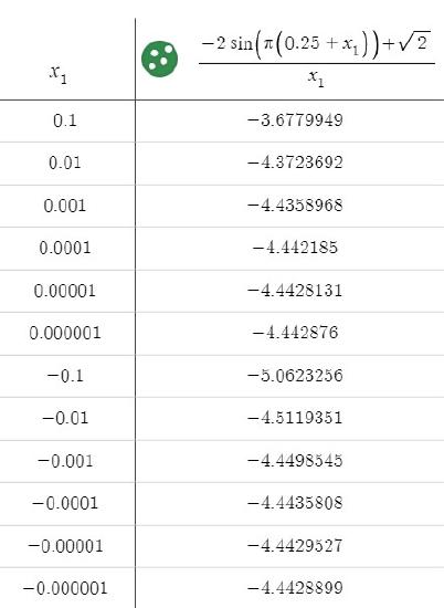
This table of values also can be built in Excel, Google Sheets, and many other applications very easily.
Footnotes
1 Leibniz defined the tangent line to a curve at a point as the line through a pair of infinitely close points on the curve.