2.10: Linear Approximations and Differentials

Learning Objectives Describe the linear approximation to a function at a point. Write the linearization of a given function. Draw a graph that illustrates the use of differentials to approximate the change in a quantity. Calculate the relative and percentage error when using a differential approximation.

Hawk A.I. Section-Specific Tutor Please note that, to access the Hawk A.I. Tutor, you will need a (free) OpenAI account.

We have just seen how derivatives allow us to compare related quantities that change over time. In this section, we examine another application of derivatives: the ability to approximate functions locally by linear functions. Linear functions are the most straightforward functions to work with, so they provide a valuable tool for approximating function values. In addition, the ideas presented in this section are generalized later in the text when we study how to approximate functions by higher-degree polynomials using Taylor Polynomial Expansions.

Linear Approximation of a Function at a Point

Consider a function $f$ that is differentiable at a point $x=a$. The tangent line to $f$ at the point $(a , f(a))$ is $$y - f(a) = f^{\prime}(a) (x - a) \implies y = f(a) + f^{\prime}(a) (x - a). \nonumber$$ For example, consider the function $f(x)=\frac{1}{x}$ at $a=2$. Since $f$ is differentiable at $x=2$ and $f^{\prime}(x)=−\frac{1}{x^2}$, we see that $f^{\prime}(2)=−\frac{1}{4}$. Therefore, the tangent line to the graph of $f$ at $a=2$ is given by the equation $$y=\dfrac{1}{2}−\dfrac{1}{4}(x−2). \nonumber$$ Figure $\PageIndex{1a}$ shows a graph of $f(x)=\frac{1}{x}$ along with the tangent line to $f$ at $x=2$. Note that for $x$ near $2$, the graph of the tangent line is close to the graph of $f$. As a result, we can use the equation of the tangent line to approximate $f(x)$ for $x$ near $2$. For example, if $x=2.1$, the $y$ value of the corresponding point on the tangent line is $$y=\dfrac{1}{2}−\dfrac{1}{4}(2.1−2)=0.475. \nonumber$$ The actual value of $f(2.1)$ is given by $$f(2.1)=\dfrac{1}{2.1} \approx 0.47619. \nonumber$$ Therefore, the tangent line gives us a fairly good approximation of $f(2.1)$ (Figure $\PageIndex{1b}$). However, note that for values of $x$ far from $2$, the equation of the tangent line does not give us a good approximation. For example, if $x=10$, the $y$-value of the corresponding point on the tangent line is $$y=\dfrac{1}{2}−\dfrac{1}{4}(10−2)=\dfrac{1}{2}−2=−1.5, \nonumber$$ whereas the value of the function at $x=10$ is $f(10)=0.1.$

Figure $\PageIndex{1a}$: The tangent line to $f(x)=1/x$ at $x=2$ provides a good approximation to $f$ for $x$ near $2$.
Figure $\PageIndex{ 1b }$: At $x=2.1$, the value of $y$ on the tangent line to $f(x)=1/x$ is $0.475$. The actual value of $f(2.1)$ is $1/2.1$, which is approximately $0.47619$.

In general, for a differentiable function $f$, the equation of the tangent line to $f$ at $x=a$ can be used to approximate $f(x)$ for $x$ near $a$. Therefore, we can write $$f(x) \approx f(a)+f^{\prime}(a)(x−a) \text{ for }x \text{ near }a.\nonumber$$ We call the linear function $$L(x)=f(a)+f^{\prime}(a)(x−a) \label{linearapprox}$$ the linear approximation, or tangent line approximation, of $f$ at $x=a$. This function $L$ is also known as the linearization of $f$ at $x=a.$

To show how beneficial the linear approximation can be, we look at how to find the linear approximation for $f(x)=\sqrt{x}$ at $x=9.$

Example $\PageIndex{1}$: Linear Approximation of $\sqrt{x}$

Find the linear approximation of $f(x)=\sqrt{x}$ at $x=9$ and use the approximation to estimate $\sqrt{9.1}$.

Solution

Since we are looking for the linear approximation at $x=9,$ using Equation $\ref{linearapprox}$ we know the linear approximation is given by $$L(x)=f(9)+f^{\prime}(9)(x−9). \nonumber$$ We need to find $f(9)$ and $f^{\prime}(9)$. $$f(x)=\sqrt{x} \implies f(9)=\sqrt{9}=3\nonumber$$ and $$f^{\prime}(x)=\dfrac{1}{2\sqrt{x}} \implies f^{\prime}(9)=\dfrac{1}{2\sqrt{9}}=\dfrac{1}{6}.\nonumber$$ Therefore, the linear approximation is given by Figure $\PageIndex{2}$. $$L(x)=3+\dfrac{1}{6}(x−9) \nonumber$$ Using the linear approximation, we can estimate $\sqrt{9.1}$ by writing $$\sqrt{9.1}=f(9.1) \approx L(9.1)=3+\dfrac{1}{6}(9.1−9) \approx 3.0167. \nonumber$$

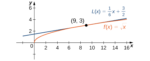
Figure $\PageIndex{2}$: The local linear approximation to $f(x)=\sqrt{x}$ at $x=9$ provides an approximation to $f$ for $x$ near $9$.

Analysis

Using a calculator, the value of $\sqrt{9.1}$ to four decimal places is $3.0166$. The value given by the linear approximation, $3.0167$, is very close to the value obtained with a calculator, so it appears that using this linear approximation is a good way to estimate $\sqrt{x}$, at least for $x$ near $9$. At the same time, it may seem odd to use a linear approximation when we can push a few buttons on a calculator to evaluate $\sqrt{9.1}$. However, how does the calculator evaluate $\sqrt{9.1}$? The calculator uses an approximation! Calculators and computers always use approximations to evaluate mathematical expressions; they just use higher-degree approximations.

Checkpoint $\PageIndex{1}$

Find the local linear approximation to $f(x)=\sqrt[3]{x}$ at $x=8$. Use it to approximate $\sqrt[3]{8.1}$ to five decimal places.

Answer

$L(x)=2+\frac{1}{12}(x−8);$ $2.00833$

Example $\PageIndex{2}$: Linear Approximation of $\sin x$

Find the linear approximation of $f(x)=\sin{(x)}$ at $x=\frac{\pi}{3}$ and use it to approximate $\sin(62^{\circ}).$

Solution

First, we recall that degree measure and calculus do not work well together. Therefore, we trade out $60^{\circ}$ for $\frac{\pi}{3}$ radians. The linear approximation is given by $$L(x)=f\left(\dfrac{\pi}{3}\right)+f^{\prime}\left(\dfrac{\pi}{3}\right)\left(x−\dfrac{\pi}{3}\right).\nonumber$$ We see that $$f(x)=\sin{(x)} \implies f\left(\dfrac{\pi}{3}\right) = \sin{\left(\dfrac{\pi}{3}\right)} = \dfrac{\sqrt{3}}{2}\nonumber$$ $$f^{\prime}(x) = \cos{(x)} \implies f^{\prime}\left(\dfrac{\pi}{3}\right) = \cos{\left(\dfrac{\pi}{3}\right)} = \dfrac{1}{2}\nonumber$$ Therefore, the linear approximation of $f$ at $x=\pi/3$ is given by Figure $\PageIndex{3}$. $$L(x) = \dfrac{\sqrt{3}}{2} + \dfrac{1}{2}\left(x−\dfrac{\pi}{3}\right)\nonumber$$ To estimate $\sin{(62^{\circ})}$ using $L$, we must first convert $62^{\circ}$ to radians. We have $62^{\circ} = \frac{62\pi}{180}$ radians, so the estimate for $\sin{(62^{\circ})}$ is given by $$\sin{(62^{\circ})} = f\left(\dfrac{62\pi}{180}\right) \approx L\left(\dfrac{62\pi}{180}\right) = \dfrac{\sqrt{3}}{2} + \dfrac{1}{2}\left(\dfrac{62\pi}{180}−\dfrac{\pi}{3}\right) = \dfrac{\sqrt{3}}{2} + \dfrac{1}{2}\left(\dfrac{2\pi}{180}\right) = \dfrac{\sqrt{3}}{2}+\dfrac{\pi}{180} \approx 0.88348.\nonumber$$

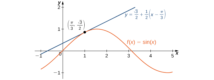
Figure $\PageIndex{3}$: The linear approximation to $f(x)=\sin x$ at $x= \pi /3$ provides an approximation to $\sin x$ for $x$ near $\pi /3.$

Checkpoint $\PageIndex{2}$

Find the linear approximation for $f(x)=\cos x$ at $x=\frac{ \pi }{2}.$

Answer

$L(x)=−x+\frac{ \pi }{2}$

Linear approximations may be used in estimating roots and powers. In the next example, we find the linear approximation for $f(x)=(1+x)^n$ at $x=0$, which can be used to estimate roots and powers for real numbers near $1$. The same idea can be extended to a function of the form $f(x)=(m+x)^n$ to estimate roots and powers near a different number $m$.

Example $\PageIndex{3}$: Approximating Roots and Powers

Find the linear approximation of $f(x)=(1+x)^n$ at $x=0$. Use this approximation to estimate $(1.01)^3.$

Solution

The linear approximation at $x=0$ is given by $$L(x) = f(0)+f^{\prime}(0)(x−0).\nonumber$$ Because $$f(x)=(1+x)^n \implies f(0)=1\nonumber$$ $$f^{\prime}(x)=n(1+x)^{n−1} \implies f^{\prime}(0)=n,\nonumber$$ the linear approximation is given by Figure $\PageIndex{4a}$. $$L(x) = 1+n(x−0) = 1+nx\nonumber$$ We can approximate $(1.01)^3$ by evaluating $L(0.01)$ when $n=3$. We conclude that $$(1.01)^3 = f(1.01) \approx L(1.01) = 1+3(0.01) = 1.03.\nonumber$$

Figure $\PageIndex{4a}$: The linear approximation of $f(x)$ at $x=0$ is $L(x)$.
Figure $\PageIndex{ 4b }$: The actual value of $1.01^3$ is $1.030301$. The linear approximation of $f(x)$ at $x=0$ estimates $1.01^3$ to be $1.03$.

Common Mistake

In Example $\PageIndex{3}$, we linearized the function $f(x) = (1 + x)^3$ at $x = 0$ to approximate $(1.01)^3$. In this case, $(1.01)^3 = f(0.01) \approx L(0.01)$. It's common for students to make the mistake of thinking, to approximate $(1.01)^3$, we need to evaluate $f$ (and, therefore, $L$) at $1.01$; however, $f(x) = (1 + x)^3$ already has the $1$ (also known as the whole part) built-in. Therefore, we need to evaluate $f$ (and, therefore, $L$) at the decimal part.

Checkpoint $\PageIndex{3}$

Find the linear approximation of $f(x)=(1+x)^4$ at $x=0$ without using the result from the preceding example.

Answer

$L(x)=1+4x$

Differentials

We have seen that linear approximations can be used to estimate function values. They can also be used to estimate the amount a function value changes due to a small change in the input. To discuss this more formally, we define a related concept: differentials. Differentials provide us with a way of estimating the amount a function changes due to a small change in input values.

When we first looked at derivatives, we used the Leibniz notation $dy/dx$ to represent the derivative of $y$ with respect to $x$. Although we used the expressions $dy$ and $dx$ in this notation, they did not have meaning on their own. Here, we see a meaning to the expressions $dy$ and $dx$. Suppose $y=f(x)$ is a differentiable function. Let $dx$ be an independent variable that can be assigned any nonzero real number, and define the dependent variable $dy$ by $$dy=f^{\prime}(x)\, dx. \label{diffeq}$$ The expressions $dy$ and $dx$ are called differentials. It is important to notice that $dy$ is a function of both $x$ and $dx$.

Example $\PageIndex{4}$: Computing Differentials

For each of the following functions, find $dy$ and evaluate when $x=3$ and $dx=0.1.$

1. $y=x^2+2x$
2. $y=\cos x$

Solutions

The key step is calculating the derivative. We can obtain $dy$ directly when we have that.

1. Since $f(x)=x^2+2x,$ we know $f^{\prime}(x)=2x+2$, and therefore $$dy=(2x+2)\,dx.\nonumber$$ When $x=3$ and $dx=0.1,$ $$dy=(2 \cdot 3+2)(0.1)=0.8.\nonumber$$
2. Since $f(x)=\cos x , f^{\prime}(x)=−\sin(x).$ This gives us $$dy=−\sin x \,dx.\nonumber$$ When $x=3$ and $dx=0.1,$ $$dy=−\sin(3)(0.1)=−0.1\sin(3).\nonumber$$

Checkpoint $\PageIndex{4}$

For $y=e^{x^2}$, find $dy$.

Answer

$dy=2xe^{x^2}dx$

We now connect differentials to linear approximations. Differentials can be used to estimate the change in the value of a function resulting from a small change in input values. Consider a function $f$ that is differentiable at point $a$. Suppose the input $x$ changes by a small amount. We are interested in how much the output $y$ changes. If $x$ changes from $a$ to $a+dx$, then the change in $x$ is $dx$ (also denoted $\Delta x$), and the change in $y$ is given by $$\Delta y=f(a+dx)−f(a). \nonumber$$ Instead of calculating the exact change in $y$, however, it is often easier to approximate the change in $y$ by using a linear approximation. For $x$ near $a, f(x)$ can be approximated by the linear approximation (Equation $\ref{linearapprox}$) $$L(x)=f(a)+f^{\prime}(a)(x−a). \nonumber$$ Therefore, if $dx$ is small, $$f(a+dx) \approx L(a+dx)=f(a)+f^{\prime}(a)(a+dx−a). \nonumber$$ That is, $$f(a+dx)−f(a) \approx L(a+dx)−f(a)=f^{\prime}(a)\,dx. \nonumber$$ In other words, the actual change in the function $f$ if $x$ increases from $a$ to $a+dx$ is approximately the difference between $L(a+dx)$ and $f(a)$, where $L(x)$ is the linear approximation of $f$ at $a$. By definition of $L(x)$, this difference is equal to $f^{\prime}(a)\,dx$. In summary, $$\Delta y=f(a+dx)−f(a) \approx L(a+dx)−f(a)=f^{\prime}(a)\,dx=dy. \nonumber$$ Therefore, we can use the differential $dy=f^{\prime}(a)\,dx$ to approximate the change in $y$ if $x$ increases from $x=a$ to $x=a+dx$. We can see this in the following graph.

Figure $\PageIndex{5}$: The differential $dy=f^{\prime}(a)\,dx$ is used to approximate the actual change in $y$ if $x$ increases from $a$ to $a+dx$.

We now look at how to use differentials to approximate the change in the value of the function that results from a small change in the value of the input. Note that the calculation with differentials is much simpler than calculating actual values of functions, and the result is very close to what we would obtain with a more exact calculation.

Example $\PageIndex{5}$: Approximating Change with Differentials

Let $y=x^2+2x.$ Compute $\Delta y$ and $dy$ at $x=3$ if $dx=0.1.$

Solution

The actual change in $y$ if $x$ changes from $x=3$ to $x=3.1$ is given by $$\Delta y=f(3.1)−f(3)=[(3.1)^2+2(3.1)]−[3^2+2(3)]=0.81.\nonumber$$ The approximate change in $y$ is given by $dy=f^{\prime}(3)\,dx$. Since $f^{\prime}(x)=2x+2,$ we have $$dy=f^{\prime}(3)\,dx=(2(3)+2)(0.1)=0.8.\nonumber$$

Checkpoint $\PageIndex{5}$

For $y=x^2+2x,$ find $\Delta y$ and $dy$ at $x=3$ if $dx=0.2.$

Answer

$dy=1.6, \; \Delta y=1.64$

A Technical Aside: The Happy Accident of Leibniz's Notation

Leibniz notation is handy throughout Calculus; however, it can be confusing for students when it comes to differentials. Visually, it looks like we can divide both sides of Equation $\ref{diffeq}$ by $dx$ to arrive at $$\dfrac{dy}{dx} = f^{\prime}(x),\nonumber$$ however, this equivalence is a happy accident.

Technically speaking, $\frac{d}{dx}$ is an operator. That is, it is a set of instructions that accepts a function and returns the derivative of that function. For example, $\frac{d}{dx} \left( y \right) = \frac{dy}{dx}$ is the operator that returns the derivative of the function $y$ with respect to $x$; however, to say that you can "pull apart" the operator and multiply both sides by $dx$ to get $dy = f^{\prime}(x) dx$ is an abuse of logic. Notationally, it works, but to be clear, it is not true that we are multiplying both sides by $dx$. $$\dfrac{dy}{dx} \text{ is }\textbf{defined}\text{ to be } f^{\prime}(x). \nonumber$$ Whereas, $$dy \text{ is }\textbf{defined}\text{ to be } f^{\prime}(x) dx. \nonumber$$ As a simple clarification, you have dealt with operators your entire life. For example, $+$ is an operator that accepts two numbers and returns the sum of those two numbers. Therefore, $3 + 2 = 5$ is true because the operator, $+$, returns the sum of $3$ and $2$ (which is $5$). I hope you would agree that "pulling apart" the operator and dividing by a "piece" of the operator to get $$3 | - 2 = 5 \implies 3 | 2 = \dfrac{5}{-} \nonumber$$ leads to a breakdown in logic (and notation).

All of this is to say that, technically, you should not tell someone, "I see you have $dy = f^{\prime}(x) dx$. Just divide both sides by $dx$ to get the derivative $\frac{dy}{dx} = f^{\prime}(x)$." That statement is (again, very technically) an abuse of logic. Moreover, saying to your friend, "Oh, you have $\frac{dy}{dx} = f^{\prime}(x)$? Great! Just multiply both sides by $dx$ to get $dy = f^{\prime}(x) dx$," is a similar abuse in logic.

It's okay to silently view the notation this way, but you should realize this result is just a happy accident of Leibniz's notation.

Calculating the Amount of Error

Any type of measurement is prone to a certain amount of error. In many applications, certain quantities are calculated based on measurements. For example, the area of a circle is calculated by measuring the radius of the circle. An error in the measurement of the radius leads to an error in the computed value of the area. Here, we examine this type of error and study how differentials can be used to estimate the error.

Consider a function $f$ with an input that is a measured quantity. Suppose the exact value of the measured quantity is $a$, but the measured value is $a+dx$. We say the measurement error is $dx$ (or $\Delta x$). As a result, an error occurs in the calculated quantity $f(x)$. This type of error is known as a propagated error and is given by $$\Delta y=f(a+dx)−f(a). \nonumber$$ Since all measurements are prone to some error, we do not know the exact value of a measured quantity, so we cannot calculate the propagated error exactly. However, given an estimate of the accuracy of a measurement, we can use differentials to approximate the propagated error $\Delta y.$ Specifically, if $f$ is a differentiable function at $a$, the propagated error is $$\Delta y \approx dy=f^{\prime}(a)\, dx. \nonumber$$ Unfortunately, we do not know the exact value $a.$ However, we can use the measured value $a+dx,$ and estimate $$\Delta y \approx dy \approx f^{\prime}(a+dx)\,dx. \nonumber$$ In the next example, we look at how differentials can be used to estimate the error in calculating the volume of a box if we assume the measurement of the side length is made with a certain amount of accuracy.

Example $\PageIndex{6}$: Volume of a Cube

Suppose the side length of a cube is measured to be $5$ cm, but we think this could be off by at most $0.1$ cm.

1. Use differentials to estimate the error in the computed volume of the cube.
2. Compute the volume of the cube if the side length is (i) $4.9$ cm and (ii) $5.1$ cm to compare the estimated error with the actual potential error.

Solutions

1. The measurement of the side length is accurate to within $\pm 0.1$ cm. Therefore, $$−0.1 \leq dx \leq 0.1.\nonumber$$ The volume of a cube is given by $V=x^3$, which leads to $$dV=3x^2dx.\nonumber$$ Using the measured side length of $5$ cm, we can estimate that $$−3(5)^2(0.1) \leq dV \leq 3(5)^2(0.1).\nonumber$$ Therefore, $$−7.5 \leq dV \leq 7.5.\nonumber$$ That is, with our possible measurement error of $\pm 0.1$ cm, our estimation of the volume could be off by at most $\pm 7.5 \text{ cm}^3$.
2. If the side length is actually $4.9$ cm, then the volume of the cube is $$V(4.9)=(4.9)^3=117.649\text{cm}^3.\nonumber$$ If the side length is actually $5.1$ cm, then the volume of the cube is $$V(5.1)=(5.1)^3=132.651\text{cm}^3.\nonumber$$ Therefore, the actual volume of the cube is between $117.649$ and $132.651$. Since the side length is measured to be 5 cm, the computed volume is $V(5)=5^3=125.$ Therefore, the error in the computed volume is $$117.649−125 \leq \Delta V \leq 132.651−125.\nonumber$$ That is, $$−7.351 \leq \Delta V \leq 7.651.\nonumber$$ We see the estimated error $dV$ is relatively close to the actual potential error in the computed volume.

Checkpoint $\PageIndex{6}$

Estimate the error in the computed volume of a cube if the side length is measured to be $6$ cm with an accuracy of $0.2$ cm.

Answer

The volume measurement is accurate to within $21.6\,\text{cm}^3$.

The measurement error $dx\ (= \Delta x)$ and the propagated error $\Delta y$ are absolute errors. We are typically interested in the size of an error relative to the size of the quantity being measured or calculated. Given an absolute error $\Delta q$ for a particular quantity, we define the relative error as $\frac{ \Delta q}{q}$, where $q$ is the actual value of the quantity. The percentage error is the relative error expressed as a percentage. For example, if we measure the height of a ladder to be $63$ in. when the actual height is $62$ in., the absolute error is 1 in., but the relative error is $\frac{1}{62}=0.016$, or $1.6\%$. By comparison, if we measure the width of a piece of cardboard to be $8.25$ in. when the actual width is $8$ in., our absolute error is $\frac{1}{4}$ in., whereas the relative error is $\frac{0.25}{8}=\frac{1}{32}$, or $3.1\%.$ Therefore, the percentage error in the measurement of the cardboard is larger, even though $0.25$ in. is less than $1$ in.

Example $\PageIndex{7}$: Relative and Percentage Error

An astronaut using a camera measures the radius of Earth as $4000$ mi with an error of $\pm 80$ mi. Let's use differentials to estimate the relative and percentage error of using this radius measurement to calculate the volume of Earth, assuming the planet is a perfect sphere.

Solution

If the measurement of the radius is accurate to within $\pm 80,$ we have $$−80 \leq dr \leq 80.\nonumber$$ Since the volume of a sphere is given by $V=(\frac{4}{3}) \pi r^3,$ we have $$dV=4 \pi r^2dr.\nonumber$$ Using the measured radius of $4000$ mi, we can estimate $$−4 \pi (4000)^2(80) \leq dV \leq 4 \pi (4000)^2(80).\nonumber$$ To estimate the relative error, consider $\frac{dV}{V}$. Since we do not know the exact value of the volume $V$, we use the measured radius $r=4000$ mi to estimate $V$. We obtain $V \approx (\frac{4}{3}) \pi (4000)^3$. Therefore the relative error satisfies $$\dfrac{−4 \pi (4000)^2(80)}{4 \pi (4000)^3/3} \leq \dfrac{dV}{V} \leq \dfrac{4 \pi (4000)^2(80)}{4 \pi (4000)^3/3},\nonumber$$ which simplifies to $$−0.06 \leq \dfrac{dV}{V} \leq 0.06.\nonumber$$ The relative error is $0.06$ and the percentage error is $6\%$.

Checkpoint $\PageIndex{7}$

Determine the percentage error if the radius of Earth is measured to be $3950$ mi with an error of $\pm 100$ mi.

Answer

$7.6\%$