4.2: Linear Approximations and Differentials

Learning Objectives

• Describe the linear approximation to a function at a point.
• Write the linearization of a given function.
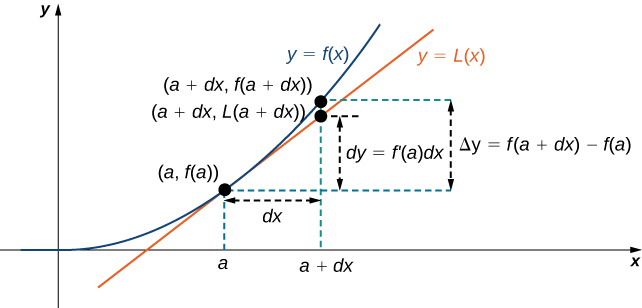
• Draw a graph that illustrates the use of differentials to approximate the change in a quantity.
• Calculate the relative error and percentage error in using a differential approximation.

We have just seen how derivatives allow us to compare related quantities that are changing over time. In this section, we examine another application of derivatives: the ability to approximate functions locally by linear functions. Linear functions are the easiest functions with which to work, so they provide a useful tool for approximating function values. In addition, the ideas presented in this section are generalized later in the text when we study how to approximate functions by higher-degree polynomials Introduction to Power Series and Functions.

Linear Approximation of a Function at a Point

Consider a function that is differentiable at a point . Recall that the tangent line to the graph of at is given by the equation

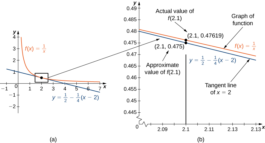
For example, consider the function at . Since is differentiable at and , we see that . Therefore, the tangent line to the graph of at is given by the equation

Figure shows a graph of along with the tangent line to at . Note that for near , the graph of the tangent line is close to the graph of . As a result, we can use the equation of the tangent line to approximate for near . For example, if , the value of the corresponding point on the tangent line is

The actual value of is given by

Therefore, the tangent line gives us a fairly good approximation of (Figure ). However, note that for values of far from , the equation of the tangent line does not give us a good approximation. For example, if , the -value of the corresponding point on the tangent line is

whereas the value of the function at is

Figure : (a) The tangent line to at provides a good approximation to for near . (b) At , the value of on the tangent line to is . The actual value of is , which is approximately .

In general, for a differentiable function , the equation of the tangent line to at can be used to approximate for near . Therefore, we can write

for near .

We call the linear function

the linear approximation, or tangent line approximation, of at . This function is also known as the linearization of at

To show how useful the linear approximation can be, we look at how to find the linear approximation for at

Example : Linear Approximation of

Find the linear approximation of at and use the approximation to estimate .

Solution

Since we are looking for the linear approximation at using Equation we know the linear approximation is given by

We need to find and

Therefore, the linear approximation is given by Figure .

Using the linear approximation, we can estimate by writing

Figure : The local linear approximation to at provides an approximation to for near .

Analysis

Using a calculator, the value of to four decimal places is . The value given by the linear approximation, , is very close to the value obtained with a calculator, so it appears that using this linear approximation is a good way to estimate , at least for x near . At the same time, it may seem odd to use a linear approximation when we can just push a few buttons on a calculator to evaluate . However, how does the calculator evaluate ? The calculator uses an approximation! In fact, calculators and computers use approximations all the time to evaluate mathematical expressions; they just use higher-degree approximations.

Exercise

Find the local linear approximation to at . Use it to approximate to five decimal places.

Hint

Answer

Example : Linear Approximation of

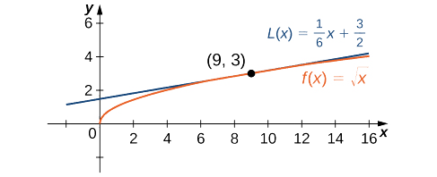
Find the linear approximation of at and use it to approximate

Solution

First we note that since rad is equivalent to , using the linear approximation at seems reasonable. The linear approximation is given by

We see that

Therefore, the linear approximation of at is given by Figure .

To estimate using , we must first convert to radians. We have radians, so the estimate for is given by

Figure : The linear approximation to at provides an approximation to for near

Exercise

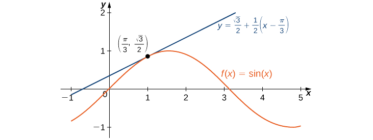
Find the linear approximation for at

Hint

Answer

Linear approximations may be used in estimating roots and powers. In the next example, we find the linear approximation for at , which can be used to estimate roots and powers for real numbers near . The same idea can be extended to a function of the form to estimate roots and powers near a different number .

Example : Approximating Roots and Powers

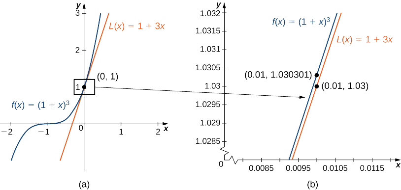
Find the linear approximation of at . Use this approximation to estimate

Solution

The linear approximation at is given by

Because

the linear approximation is given by Figure .

We can approximate by evaluating when . We conclude that

Figure : (a) The linear approximation of at is . (b) The actual value of is . The linear approximation of at estimates to be .

Exercise

Find the linear approximation of at without using the result from the preceding example.

Hint

Answer

Differentials

We have seen that linear approximations can be used to estimate function values. They can also be used to estimate the amount a function value changes as a result of a small change in the input. To discuss this more formally, we define a related concept: differentials. Differentials provide us with a way of estimating the amount a function changes as a result of a small change in input values.

When we first looked at derivatives, we used the Leibniz notation to represent the derivative of with respect to . Although we used the expressions and in this notation, they did not have meaning on their own. Here we see a meaning to the expressions and . Suppose is a differentiable function. Let be an independent variable that can be assigned any nonzero real number, and define the dependent variable by

It is important to notice that is a function of both and . The expressions and are called differentials. We can divide both sides of Equation by which yields

This is the familiar expression we have used to denote a derivative. Equation is known as the differential form of Equation .

Example : Computing Differentials

For each of the following functions, find and evaluate when and

Solution

The key step is calculating the derivative. When we have that, we can obtain directly.

a. Since we know , and therefore

When and

b. Since This gives us

When and

Exercise

For , find .

Hint

Answer

We now connect differentials to linear approximations. Differentials can be used to estimate the change in the value of a function resulting from a small change in input values. Consider a function that is differentiable at point . Suppose the input changes by a small amount. We are interested in how much the output changes. If changes from to , then the change in is (also denoted ), and the change in is given by

Instead of calculating the exact change in , however, it is often easier to approximate the change in by using a linear approximation. For near can be approximated by the linear approximation (Equation )

Therefore, if is small,

That is,

In other words, the actual change in the function if increases from to is approximately the difference between and , where is the linear approximation of at . By definition of , this difference is equal to . In summary,

Therefore, we can use the differential to approximate the change in if increases from to . We can see this in the following graph.

Figure : The differential is used to approximate the actual change in if increases from to .

We now take a look at how to use differentials to approximate the change in the value of the function that results from a small change in the value of the input. Note the calculation with differentials is much simpler than calculating actual values of functions and the result is very close to what we would obtain with the more exact calculation.

Example : Approximating Change with Differentials

Let Compute and at if

Solution

The actual change in if changes from to is given by

The approximate change in is given by . Since we have

Exercise

For find and at if

Hint

Answer

Calculating the Amount of Error

Any type of measurement is prone to a certain amount of error. In many applications, certain quantities are calculated based on measurements. For example, the area of a circle is calculated by measuring the radius of the circle. An error in the measurement of the radius leads to an error in the computed value of the area. Here we examine this type of error and study how differentials can be used to estimate the error.

Consider a function with an input that is a measured quantity. Suppose the exact value of the measured quantity is , but the measured value is . We say the measurement error is (or ). As a result, an error occurs in the calculated quantity . This type of error is known as a propagated error and is given by

Since all measurements are prone to some degree of error, we do not know the exact value of a measured quantity, so we cannot calculate the propagated error exactly. However, given an estimate of the accuracy of a measurement, we can use differentials to approximate the propagated error Specifically, if is a differentiable function at ,the propagated error is

Unfortunately, we do not know the exact value However, we can use the measured value and estimate

In the next example, we look at how differentials can be used to estimate the error in calculating the volume of a box if we assume the measurement of the side length is made with a certain amount of accuracy.

Example : Volume of a Cube

Suppose the side length of a cube is measured to be cm with an accuracy of cm.

1. Use differentials to estimate the error in the computed volume of the cube.
2. Compute the volume of the cube if the side length is (i) cm and (ii) cm to compare the estimated error with the actual potential error.

Solution

a. The measurement of the side length is accurate to within cm. Therefore,

The volume of a cube is given by , which leads to

Using the measured side length of cm, we can estimate that

Therefore,

b. If the side length is actually cm, then the volume of the cube is

If the side length is actually cm, then the volume of the cube is

Therefore, the actual volume of the cube is between and . Since the side length is measured to be 5 cm, the computed volume is Therefore, the error in the computed volume is

That is,

We see the estimated error is relatively close to the actual potential error in the computed volume.

Exercise

Estimate the error in the computed volume of a cube if the side length is measured to be cm with an accuracy of cm.

Hint

Answer

The volume measurement is accurate to within .

The measurement error and the propagated error are absolute errors. We are typically interested in the size of an error relative to the size of the quantity being measured or calculated. Given an absolute error for a particular quantity, we define the relative error as , where is the actual value of the quantity. The percentage error is the relative error expressed as a percentage. For example, if we measure the height of a ladder to be in. when the actual height is in., the absolute error is 1 in. but the relative error is , or . By comparison, if we measure the width of a piece of cardboard to be in. when the actual width is in., our absolute error is in., whereas the relative error is , or Therefore, the percentage error in the measurement of the cardboard is larger, even though in. is less than in.

Example : Relative and Percentage Error

An astronaut using a camera measures the radius of Earth as mi with an error of mi. Let’s use differentials to estimate the relative and percentage error of using this radius measurement to calculate the volume of Earth, assuming the planet is a perfect sphere.

Solution: If the measurement of the radius is accurate to within we have

Since the volume of a sphere is given by we have

Using the measured radius of mi, we can estimate

To estimate the relative error, consider . Since we do not know the exact value of the volume , use the measured radius mi to estimate . We obtain . Therefore the relative error satisfies

which simplifies to

The relative error is and the percentage error is .

Exercise

Determine the percentage error if the radius of Earth is measured to be mi with an error of mi.

Hint

Use the fact that to find .

Answer

Key Concepts

• A differentiable function can be approximated at by the linear function

• For a function , if changes from to , then

is an approximation for the change in . The actual change in is

• A measurement error can lead to an error in a calculated quantity . The error in the calculated quantity is known as the propagated error. The propagated error can be estimated by

• To estimate the relative error of a particular quantity , we estimate .

Key Equations

• Linear approximation

• A differential

Glossary

differential

the differential is an independent variable that can be assigned any nonzero real number; the differential is defined to be

differential form

given a differentiable function the equation is the differential form of the derivative of with respect to

linear approximation

the linear function is the linear approximation of at

percentage error

the relative error expressed as a percentage

propagated error

the error that results in a calculated quantity resulting from a measurement error

relative error

given an absolute error for a particular quantity, is the relative error.

tangent line approximation (linearization)

since the linear approximation of at is defined using the equation of the tangent line, the linear approximation of at is also known as the tangent line approximation to at