1.1: Areas Between Curves

Note to the Instructor (click to expand) This section only covers areas between curves (with a clarification of the difference between a direct integration problem and being requested to find areas). Focus should be on requiring graphing skills (algebraic, trigonometric, exponential, etc.). To succeed in this section, you'll need to use some skills from previous courses. While you should already know them, this is the first time they've been required. You can review these skills in CRC's Corequisite Codex. If you have a support class, it might cover some, but not all, of these topics. Prerequisite Skills and Support Topics (click to expand) Geometry The Pythagorean Theorem, Distance Formula, and Midpoint Formula: The concept of distance, particularly the distance formula, is reviewed in the section as foundational for understanding $y_T - y_B$ and $x_R - x_L$. Simplifying Expressions Multiplying and Distributing Polynomial Expressions: Necessary for simplifying the integrand $f(x)-g(x)$ after substitution. Solving Equations Solving Linear Equations: Essential for finding intersection points when the bounding curves are lines. Solving Quadratic Equations: Required for finding intersection points when one or both bounding curves are quadratic functions (as seen in Example 2). Solving Polynomial Equations: Generally needed to find points where $f(x)=g(x)$ if the functions are polynomials, which define the limits of integration. Solving Radical Equations: May be needed if functions involve roots and intersections are sought, or when converting $y=f(x)$ to $x=v(y)$. Graphs The Cartesian Coordinate System and the Quadrants: Fundamental for setting up and visualizing the area problem in a 2D plane. Ordered Pairs and Graphing Relations by Point-Plotting: Essential for sketching the functions to correctly identify the region, the upper/lower or right/left functions, and the limits of integration. An Overview of Functions The Definition of a Function: Crucial for understanding the relationships $y=f(x)$ and $x=u(y)$ that define the boundaries of the area. Evaluating Functions: Necessary for finding specific points on curves, comparing function values, and for numerical approximation methods. The Domain and Range of a Function: Important for understanding the intervals over which functions are defined and where intersections might occur. Graphing Functions Graphs of Functions: The ability to sketch or visualize graphs is paramount for setting up the correct integral for the area between curves. Base Graphs: Recognizing the shapes of common functions (lines, parabolas, square roots, trigonometric functions) helps in quickly sketching the region. Trigonometry Evaluating Trigonometric Functions at Special Angles: Required for calculations when limits of integration or intersection points involve these specific angles (e.g., $\frac{\pi}{4}$). Base Graphs of the Trigonometric Functions: Important for visualizing regions bounded by trigonometric curves like sine and cosine. Solving Simple Trigonometric Equations: Necessary for finding the intersection points of trigonometric functions, which determine the limits of integration. Trigonometric Identities - The Pythagorean Identities: Often used in simplifying expressions or solving trigonometric equations. Trigonometric Identities - Sum and Difference of Angles Identities: Useful in various trigonometric manipulations. Trigonometric Identities - Double-Angle Identities: Can be needed for solving equations or simplifying integrands. Trigonometric Identities - Half-Angle and Power Reduction Identities: Particularly power reduction formulas can be useful in integration, though not directly for area setup here, they are part of the expected mastery. The following is a list of learning objectives for this section. Learning Objectives (click to expand) Determine the area of a region between two curves by integrating with respect to the independent variable. Find the area of a compound region. Determine the area of a region between two curves by integrating with respect to the dependent variable.

Hawk A.I. Section-Specific Tutor To access the Hawk A.I. Tutor, you will need to be logged into your campus Gmail account.

A Review of Necessary Prerequisite Theory

The following video is an excellent place to start before your first class meeting. It contains a review of the necessary theory from Differential Calculus (a.k.a. Calculus I) to begin your pathway to success in this course.

In Differential Calculus, we developed the definite integral concept to calculate the area between a curve and an axis on a given interval. In this section, we expand that idea to calculate the area of more complex regions. We start by finding the area between two curves that are functions of $x$, beginning with the simple case in which one function is always greater than the other. We then look at instances where the graphs of the functions cross. Lastly, we consider how to calculate the area between two curves that are functions of $y$.

An Aside: Measuring Distances

Before we dive into Integral Calculus (a.k.a., Calculus II), let's take a moment to discuss something simple and familiar - distance.¹ Specifically, we need to recall the Distance Formula. The distance between any two points, $P\left( x_1, y_1 \right)$ and $Q\left( x_2,y_2 \right)$, in the Cartesian plane is $$d\left( P,Q \right) = \sqrt{\left(x_1 - x_2\right)^2 + \left(y_1 - y_2\right)^2}. \label{DistanceFormula}$$ If the two points share the same $x$-coordinate (i.e., they lie on the same vertical line), then Equation $\ref{DistanceFormula}$ becomes $$d\left( P,Q \right) = \sqrt{\left(y_1 - y_2\right)^2} = \left| y_1 - y_2 \right| = \begin{cases} y_1 - y_2 & \text{if} & y_1 \geq y_2 \\ y_2 - y_1 & \text{if} & y_1 \lt y_2 \\ \end{cases}. \nonumber$$ This can be read as follows:

The distance between any two points on a vertical line is $y_T - y_B$, where $y_T = y_{\text{Top}} = \max\{ y_1, y_2 \}$ and $y_B = y_{\text{Bottom}} = \min\{ y_1, y_2 \}$.

This interpretation will be critical as we move forward.

If we, instead, assume that the points $P$ and $Q$ lie on the same horizontal line (thereby having the same $y$-coordinates), then Equation $\ref{DistanceFormula}$ becomes $$d\left( P,Q \right) = \sqrt{\left(x_1 - x_2\right)^2} = \left| x_1 - x_2 \right| = \begin{cases} x_1 - x_2 & \text{if} & x_1 \geq x_2 \\ x_2 - x_1 & \text{if} & x_1 \lt x_2 \\ \end{cases}. \nonumber$$ This can be read as follows:

The distance between any two points on a horizontal line is $x_R - x_L$, where $x_R = x_{\text{Right}} = \max\{ x_1, x_2 \}$ and $x_L = x_{\text{Left}} = \min\{ x_1 , x_2 \}$.

The two statements, that the distance between two points on a vertical line is $y_{\text{Top}} - y_{\text{Bottom}}$ and the distance between two points on the horizontal line is $x_{\text{Right}} - x_{\text{Left}}$, are going to be used repeatedly in this course. For example, we will often need to determine the distance between a function, say $f(x)$, and a horizontal line, say $y = L$. If we know that $L \ge f(x)$ on the interval $[a,b]$, then the vertical distance between $y = L$ and the function $f(x)$ is always going to be $y_{\text{Top}} - y_{\text{Bottom}} = L - f(x)$, for all $x \in [a,b]$. Likewise, if we know the function $g(y)$ is always to the left of $h(y)$ for $y \in [c,d]$, then the horizontal distance between these two functions for any value of $y$ in $[c,d]$ is $x_{\text{Right}} - x_{\text{Left}} = h(y) - g(y)$.

While the previous paragraph is (hopefully) simple to understand, the results are immensely helpful for us. It's now time to return to Calculus!

Area of a Region between Two Curves

Let $f(x)$ and $g(x)$ be continuous functions over an interval $[a,b]$ such that $f(x) \ge g(x)$ on $[a,b]$. We want to find the area between the graphs of the functions, as shown in Figure $\PageIndex{1}$.

Figure $\PageIndex{1}$: The area between the graphs of two functions, $f(x)$ and $g(x)$, on the interval $[a,b]$

As we did before, we will partition the interval on the $x$-axis and approximate the area between the graphs of the functions with rectangles. So, for $i=0,1,2, \ldots ,n$, let $P=\{x_i\}$ be a regular partition of $[a,b]$. Then, for $i=1,2, \ldots ,n,$ choose a point $x^∗_i \in [x_{i−1},x_i]$, and on each interval $[x_{i−1},x_i]$ construct a rectangle that extends vertically from $g(x^∗_i)$ to $f(x^∗_i)$. Figure $\PageIndex{2}$(a) shows the rectangles when $x^∗_i$ is selected to be the left endpoint of the interval and $n=10$. Figure $\PageIndex{2}$(b) shows a representative rectangle in detail.

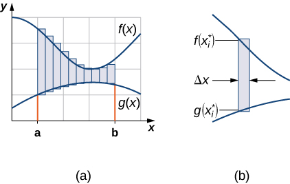
Figure $\PageIndex{2}$: (a) We can approximate the area between the graphs of two functions, $f(x)$ and $g(x)$, with rectangles. (b) The area of a typical rectangle goes from one curve to the other.

The height of each individual rectangle is $y_{T_i} - y_{B_i} = f(x^∗_i)−g(x^∗_i)$ and the width of each rectangle is $\Delta x$. Adding the areas of all the rectangles, we see that the area between the curves is approximated by $$A \approx \sum_{i=1}^n[y_{T_i} - y_{B_i}] \Delta x = \sum_{i=1}^n[f(x^∗_i)−g(x^∗_i)] \Delta x. \nonumber$$ This is a Riemann sum, so we take the limit as $n \to \infty$ and we get $$A=\lim_{n \to \infty}\sum_{i=1}^n[f(x^∗_i)−g(x^∗_i)] \Delta x=\int ^b_a[f(x)−g(x)]dx. \nonumber$$ These findings are summarized in the following theorem.

Theorem: Area between Two Curves

Let $f(x)$ and $g(x)$ be continuous functions such that $f(x) \geq g(x)$ over an interval [$a,b]$. Let $\textbf{R}$ denote the region bounded above by the graph of $f(x)$, below by the graph of $g(x)$, and on the left and right by the lines $x=a$ and $x=b$, respectively. Then, the area of $\textbf{R}$ is given by $$A=\int ^b_a[f(x)−g(x)]dx. \nonumber$$

We apply this theorem in the following example.

Example $\PageIndex{1}$

If $\textbf{R}$ is the region bounded above by the graph of the function $f(x)=x+4$ and below by the graph of the function $g(x)=3−\frac{x}{2}$ over the interval $[1,4]$, find the area of region $\textbf{R}$.

Solution

Graphing the requested region, depicted in the following figure, will be a requirement.

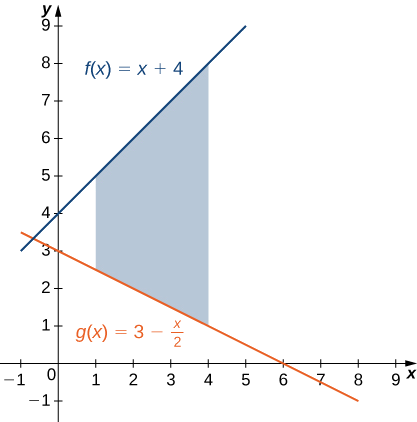
Figure $\PageIndex{3}$: A region between two curves is shown where one curve is always greater than the other.

We can see that the values of $y_T$ are always "played by" $f(x)$ and the values of $y_B$ are always "played by" $g(x)$. Therefore, we have $$\begin{array}{rcl} A & = & \displaystyle \int ^b_a[y_T − y_B]\,dx \\ \\ & = & \displaystyle \int ^b_a[f(x)−g(x)]\,dx \\ \\ & = & \displaystyle \int ^4_1 \left[(x+4)−\left(3−\dfrac{x}{2}\right) \right]\,dx \\ \\ & = & \displaystyle \int ^4_1\left[\dfrac{3x}{2}+1\right]\,dx \\ \\ & = & \left[ \dfrac{3x^2}{4}+x \right]\bigg|^4_1 \\ \\ & = & \left(16−\dfrac{7}{4}\right) \\ \\ & = & \dfrac{57}{4}. \\ \end{array} \nonumber$$ The area of the region is $\frac{57}{4} \text{ units}^2$.

Checkpoint $\PageIndex{1}$

If $\textbf{R}$ is the region bounded by the graphs of the functions $f(x)=\frac{x}{2}+5$ and $g(x)=x+\frac{1}{2}$ over the interval $[1,5]$, find the area of region $\textbf{R}$.

Answer

$12 \text{ units}^2$

In Example $\PageIndex{1}$, we defined the interval of interest as part of the problem statement. Quite often, though, we want to define our interval of interest based on where the graphs of the two functions intersect. This is illustrated in the following example.

Example $\PageIndex{2}$

If $\textbf{R}$ is the region bounded above by the graph of the function $f(x)=9−\left(\frac{x}{2}\right)^2$ and below by the graph of the function $g(x)=6−x$, find the area of region $\textbf{R}$.

Solution

The region is depicted in the following figure, and we can see that $y_T = f(x)$ and $y_B = g(x)$ over the entire region.

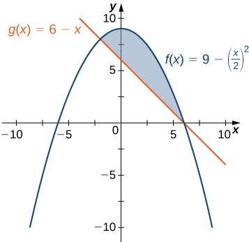
Figure $\PageIndex{4}$: This graph shows the region below the graph of $f(x)$ and above the graph of $g(x).$

We first need to compute where the graphs of the functions intersect. Setting $f(x)=g(x),$ we get $$\begin{array}{crcl} & f(x) &= & g(x) \\ \\ \implies & 9−\left(\dfrac{x}{2}\right)^2 & = & 6−x \\ \\ \implies & 9−\dfrac{x^2}{4} & = & 6−x \\ \\ \implies & 36−x^2 & = & 24−4x \\ \\ \implies & x^2−4x−12 & = & 0 \\ \\ \implies & (x−6)(x+2) & = & 0. \\ \end{array} \nonumber$$ The graphs of the functions intersect when $x=6$ or $x=−2,$ so we want to integrate from $−2$ to $6$. Therefore, $$\begin{array}{rcl} A & = & \displaystyle \int^b_a[y_T−y_B]\,dx \\ \\ & = & \displaystyle \int^b_a[f(x)−g(x)]\,dx \\ \\ & = & \displaystyle \int ^6_{−2} \left[9−\left(\dfrac{x}{2}\right)^2−(6−x)\right]\,dx \\ \\ & = & \displaystyle \int ^6_{−2}\left[3−\dfrac{x^2}{4}+x\right]\,dx \\ \\ & = & \left. \left[3x−\dfrac{x^3}{12}+\dfrac{x^2}{2}\right] \right|^6_{−2} \\ \\ & = & \dfrac{64}{3}. \\ \end{array} \nonumber$$ The area of the region is $\frac{64}{3} \text{ units}^2$.

Checkpoint $\PageIndex{2}$

If $\textbf{R}$ is the region bounded above by the graph of the function $f(x)=x$ and below by the graph of the function $g(x)=x^4$, find the area of region $\textbf{R}$.

Answer

$\frac{3}{10} \text{ units}^2$

Areas of Compound Regions

What if we want to examine regions bounded by graphs of functions that cross one another? In that case, we modify the process we just developed by using the absolute value function.

Theorem: Finding the Area of a Region between Curves That Cross

Let $f(x)$ and $g(x)$ be continuous functions over an interval $[a,b]$. Let $\textbf{R}$ denote the region between the graphs of $f(x)$ and $g(x)$, and be bounded on the left and right by the lines $x=a$ and $x=b$, respectively. Then, the area of $\textbf{R}$ is given by $$A=\int ^b_a|f(x)−g(x)|dx. \nonumber$$

In practice, applying this theorem requires us to break up the interval $[a,b]$ and evaluate several integrals, depending on which function values are greater over a given part of the interval. We study this process in the following example.

Example $\PageIndex{3}$

If $\textbf{R}$ is the region between the graphs of the functions $f(x)=\sin(x)$ and $g(x)=\cos(x)$ over the interval $[0, \pi ]$, find the area of region $\textbf{R}$.

Solution

The region is depicted in the following figure.

Figure $\PageIndex{5}$: The region between two curves can be broken into two sub-regions.

The graphs of the functions intersect at $x = \frac{\pi}{4}$. Since the roles of $y_T$ and $y_B$ switch between regions $\textbf{R}_1$ and $\textbf{R}_2$, our notation for $y_{\text{top}}$ and $y_{\text{bottom}}$ needs to gain a little more complexity.

For $x \in \left[0, \frac{\pi}{4}\right]$, $$|f(x)−g(x)| = y_{T_1} - y_{B_1} = \cos(x)−\sin(x) . \nonumber$$ On the other hand, for $x \in \left[ \frac{\pi}{4}, \pi \right]$, $$|f(x)−g(x)| = y_{T_2} - y_{B_2} = \sin(x) −\cos(x). \nonumber$$ Then $$\begin{array}{rcl} A & = & \displaystyle \int ^b_a|f(x)−g(x)|dx \\ \\ & = & \displaystyle \int ^ \pi _0|\sin(x) −\cos(x)|dx \\ \\ & = & \displaystyle \int ^{ \pi /4}_0(y_{T_1} − y_{B_1} )dx+\int ^{ \pi }_{ \pi /4}(y_{T_2} −y_{B_2})dx \\ \\ & = & \displaystyle \int ^{ \pi /4}_0(\cos(x)−\sin(x) )dx+\int ^{ \pi }_{ \pi /4}(\sin(x) −\cos(x))dx \\ \\ & = & [\sin(x) +\cos(x)] \bigg|^{ \pi /4}_0+[−\cos(x)−\sin(x) ] \bigg|^ \pi _{ \pi /4} \\ \\ & = & (\sqrt{2}−1)+(1+\sqrt{2}) \\ \\ & = & 2\sqrt{2}. \\ \end{array} \nonumber$$ The area of the region is $2\sqrt{2} \text{ units}^2$.

Caution: Mastery of Trigonometry is required in this course

Your success in Calculus II will rely heavily on your mastery of concepts from Trigonometry. You will frequently need to recall, without any prompting, the following identities and theorems:

• Pythagorean Identities,
• Sum and Difference Formulas (for sine and cosine),
• Double-Angle Identities (for sine and cosine),
• Half-Angle Formulas (for sine and cosine) - these are also known as the Power Reduction Formulas, and
• the Even/Odd Identities.

Moreover, it is assumed you can perform each of the following skills without using technology for help:

• evaluate all trigonometric functions at special angles, or at angles having special angles as reference angles, as well as at axial angles,
• accurately graph transformations of trigonometric functions,
• solve trigonometric equations,
• evaluate inverse trigonometric functions,
• understand the domain and range restrictions of all base trigonometric functions, and
• understand the domain and range restrictions of all base inverse trigonometric functions.

If you need a quick review of your Trigonometry, please see Section 1.6 of the Differential Calculus textbook. If you need a deeper review, an entire course in Trigonometry (i.e., Math 373 at CRC) is a great choice.

Checkpoint $\PageIndex{3}$

If $\textbf{R}$ is the region between the graphs of the functions $f(x)=\sin(x)$ and $g(x)=\cos(x)$ over the interval $\left[ \frac{\pi}{2},2 \pi \right]$, find the area of region $\textbf{R}$.

Answer

$2+2\sqrt{2} \text{ units}^2$

Example $\PageIndex{4}$

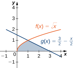
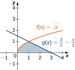
Consider the region depicted in Figure $\PageIndex{6}$. Find the area of $\textbf{R}$.

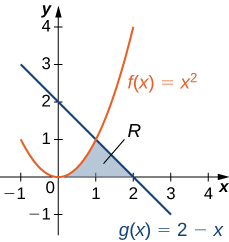
Figure $\PageIndex{6}$: Two integrals are required to calculate the area of this region.

Solution

As with Example $\PageIndex{3}$, we need to divide the interval into two pieces. The graphs of the functions intersect at $x=1$ (set $f(x)=g(x)$ and solve for $x$), so we evaluate two separate integrals: one over the interval $[0,1]$ and one over the interval $[1,2]$.

Over the interval $[0,1]$, the region is bounded above by $y_{T_1} = f(x) = x^2$ and below by $y_{B_1} = 0$, which is the $x$-axis, so we have $$A_1=\int ^1_0\left( y_{T_1} - y_{B_1} \right)dx=\int ^1_0(x^2 - 0)dx=\int ^1_0x^2 dx= \dfrac{x^3}{3} \bigg|^1_0=\dfrac{1}{3}. \nonumber$$ Over the interval $[1,2],$ the region is bounded above by $y_{T_2} = g(x)=2−x$ and below by $y_{B_2} = 0$, which again is the $x$-axis, so we have $$A_2=\int ^2_1\left( y_{T_2} - y_{B_2} \right)dx=\int ^2_1(2−x - 0)dx=\int ^2_1(2−x)dx=\left[2x−\dfrac{x^2}{2}\right]\bigg|^2_1=\dfrac{1}{2}. \nonumber$$ Adding these areas together, we obtain $$A=A_1+A_2=\dfrac{1}{3}+\dfrac{1}{2}=\dfrac{5}{6}.\nonumber$$ The area of the region is $\frac{5}{6} \text{ units}^2$.

Checkpoint $\PageIndex{4}$

Consider the region depicted in the following figure. Find the area of $\textbf{R}$.

Answer

$\frac{5}{3} \text{ units}^2$

Regions Defined with Respect to $y$

In Example $\PageIndex{4}$, we had to evaluate two separate integrals to calculate the area of the region. However, there is another approach that requires only one integral. What if we treat the curves as functions of $y$ instead of as functions of $x$? Review Figure $\PageIndex{6}$. Note that the left graph, shown in red, is represented by the function $y=f(x)=x^2$. We could just as easily solve this for $x$ and represent the curve by the function of $y$, $x=v(y)=\sqrt{y}$.² Similarly, the right graph is represented by the function $y=g(x)=2−x$, but could just as easily be represented by the function $x=u(y)=2−y$. When the graphs are represented as functions of $y$, we see the region is bounded on the left by the graph of one function and on the right by the graph of the other function. Therefore, if we integrate with respect to $y$, we only need to evaluate one integral. Let’s develop a formula for this type of integration.

Let $u(y)$ and $v(y)$ be continuous functions over an interval $[c,d]$ such that $u(y) \geq v(y)$ for all $y \in [c,d]$. We want to find the area between the graphs of the functions, as shown in Figure $\PageIndex{7}$.

Figure $\PageIndex{7}$: We can find the area between the graphs of two functions, $u(y)$ and $v(y)$.

This time, we are going to partition the interval on the $y$-axis and use horizontal rectangles to approximate the area between the functions. So, for $i=0,1,2, \ldots ,n$, let $Q=\{y_i\}$ be a regular partition of $[c,d]$. Then, for $i=1,2, \ldots ,n$, choose a point $y^∗_i \in [y_{i−1},y_i]$, then over each interval $[y_{i−1},y_i]$ construct a rectangle that extends horizontally from $v(y^∗_i)$ to $u(y^∗_i)$. Figure $\PageIndex{8}$(a) shows the rectangles when $y^∗_i$ is selected to be the lower endpoint of the interval and $n=10$. Figure $\PageIndex{8}$(b) shows a representative rectangle in detail.

Figure $\PageIndex{8}$: (a) Approximating the area between the graphs of two functions, $u(y)$ and $v(y)$, with rectangles. (b) The area of a typical rectangle.

The height of each individual rectangle is $\Delta y$ and the width of each rectangle is $x_{R_i} - x_{L_i} = u(y^∗_i)−v(y^∗_i)$. Therefore, the area between the curves is approximately $$A \approx \sum_{i=1}^n[x_{R_i} - x_{L_i}] \Delta y = \sum_{i=1}^n[u(y^∗_i)−v(y^∗_i)] \Delta y . \nonumber$$ This is a Riemann sum, so we take the limit as $n \to \infty,$ obtaining $$\begin{array}{rcl} A & = & \displaystyle \lim_{n \to \infty}\sum_{i=1}^n[x_{R_i} - x_{L_i}] \Delta y \\ \\ & = & \displaystyle \lim_{n \to \infty}\sum_{i=1}^n[u(y^∗_i)−v(y^∗_i)] \Delta y \\ \\ & = & \displaystyle \int ^d_c[u(y)−v(y)]dy. \\ \end{array} \nonumber$$ These findings are summarized in the following theorem.

Theorem: Finding the Area between Two Curves, Integrating along the $y$-axis

Let $u(y)$ and $v(y)$ be continuous functions such that $u(y) \geq v(y)$ for all $y \in [c,d]$. Let $\textbf{R}$ denote the region bounded on the right by the graph of $u(y)$, on the left by the graph of $v(y)$, and above and below by the lines $y=d$ and $y=c$, respectively. Then, the area of $\textbf{R}$ is given by $$A=\int ^d_c[u(y)−v(y)]dy. \nonumber$$

Example $\PageIndex{5}$

Let’s revisit Example $\PageIndex{4}$; only this time, let’s integrate with respect to $y$. Let $\textbf{R}$ be the region depicted in Figure $\PageIndex{9}$. Find the area of $\textbf{R}$ by integrating with respect to $y$.

Figure $\PageIndex{9}$: The area of region $\textbf{R}$ can be calculated using one integral only when the curves are treated as functions of $y$.

Solution

We must first express the graphs as functions of $y$. As we saw at the beginning of this section, the curve on the left can be represented by the function $x_L=v(y)=\sqrt{y}$, and the curve on the right can be represented by the function $x_R=u(y)=2−y$.

Now, we have to determine the limits of integration. The region is bounded below by the $x$-axis, so the lower limit of integration is $y=0$. The upper limit of integration is determined by the point where the two graphs intersect, which is the point $(1,1)$, so the upper limit of integration is $y=1$. Thus, we have $[c,d]=[0,1]$.

Calculating the area of the region, we get $$\begin{array}{rcl} A & = & \displaystyle \int ^d_c[x_R - x_L]dy \\ \\ & = & \displaystyle \int ^d_c[u(y)−v(y)]dy \\ \\ & = & \displaystyle \int ^1_0[(2−y)−\sqrt{y}]dy \\ \\ & = & \left[2y−\dfrac{y^2}{2}−\dfrac{2}{3}y^{3/2}\right] \bigg|^1_0\\ \\ & = & \dfrac{5}{6}. \\ \end{array} \nonumber$$ The area of the region is $\frac{5}{6} \text{ units}^2$.

Caution: Understand the meaning of $\left| f(x) - g(x) \right|$

While the notations, $y_T$, $y_B$, $x_R$, and $x_L$ are incredibly helpful in properly setting up integrals to determine areas between curves (and, later, for rotational volumes), you are not excused from understanding the true definition of $\left| f(x) - g(x) \right|$.

Checkpoint $\PageIndex{5}$

Let’s revisit Checkpoint $\PageIndex{4}$; only this time, let’s integrate with respect to $y$. Let $\textbf{R}$ be the region depicted in the following figure. Find the area of $\textbf{R}$ by integrating with respect to $y$.

Answer

$\frac{5}{3} \text{ units}^2$

Approximating Areas Between Curves

We can combine concepts from Calculus I with our new knowledge to approximate the area between two curves.

Example $\PageIndex{6}$

Approximate the area between $f(x) = \cosh(x)$ and $g(x) = - \frac{x}{2x^2 + 1}$ on the interval $[-2,2]$ using vertical slices and right endpoints with $n = 8$.

Solution

First, it is actually possible for us to compute the exact area between these two curves. Consider the Figure $\PageIndex{10}$ below.

Figure $\PageIndex{10}$

We can easily see that the area can be computed using the definite integral $$\begin{array}{rclr} A & = & \displaystyle \int_{-2}^{2} \left( y_T - y_B \right) dx & \\ \\ & = & \displaystyle \int_{-2}^{2} \left( f(x) - g(x) \right) dx & \\ \\ & = & \displaystyle \int_{-2}^{2} \left( \cosh(x) + \dfrac{x}{2x^2 + 1} \right) dx & \\ \\ & = & \displaystyle \int_{-2}^{2} \cosh(x) dx + \int_{-2}^{2} \dfrac{x}{2x^2 + 1} dx & \\ \\ & = & \displaystyle \int_{-2}^{2} \cosh(x) dx + 0 & \left( \dfrac{x}{2x^2 + 1} \text{ is an odd function being integrated over a symmetric interval.} \right) \\ \\ & = & 2 \displaystyle \int_{0}^{2} \cosh(x) dx & \left( \cosh(x) \text{ is an even function being integrated over a symmetric interval.} \right) \\ \\ & = & 2 \sinh(x) \bigg|_{0}^{2} & \\ \\ & = & 2 \sinh(2) - 2\sinh(0) & \\ \\ & = & 2 \sinh(2) - 0 & \\ \\ & = & 2 \sinh(2) & \\ \end{array} \nonumber$$ However, we are being asked to approximate the value of this area, so let's practice our skills from Calculus I.

We are given $n = 8$, which implies $\Delta x = \frac{b - a}{n} = \frac{2 - (-2)}{8} = \frac{1}{2}$ and $x_i = a + i \Delta x = -2 + \frac{1}{2}i$. Therefore, $$\begin{array}{rcl} A & \approx & R_8 \\ \\ & = & \displaystyle \sum_{i = 1}^{8} \left( y_{T_i} - y_{B_i} \right) \Delta x \\ \\ & = & \displaystyle \sum_{i = 1}^{8} \left( f(x_i) - g(x_i) \right) \Delta x \\ \\ & = & \displaystyle \sum_{i = 1}^{8} \left( f\left(-2 + \dfrac{1}{2} i\right) - g\left(-2 + \dfrac{1}{2} i\right) \right) \dfrac{1}{2} \\ \\ & = & \dfrac{1}{2} \displaystyle \sum_{i = 1}^{8} \left( \cosh\left(-2 + \dfrac{1}{2} i\right) + \frac{-2 + \dfrac{1}{2} i}{2\left(-2 + \dfrac{1}{2} i\right)^2 + 1} \right) \\ \\ & = & \dfrac{1}{2} \left\{ \left[ \cosh\left( -\dfrac{3}{2} \right) + \dfrac{-\frac{3}{2}}{2 \left( -\frac{3}{2} \right)^2 + 1} \right] + \left[ \cosh\left( -1 \right) + \dfrac{-1}{2 \left( -1 \right)^2 + 1} \right] + \cdots + \left[ \cosh\left( 2 \right) + \dfrac{2}{2 \left( 2 \right)^2 + 1} \right] \right\} \\ \\ & \approx & 7.5153 \\ \end{array} \nonumber$$

Advice: Review hyperbolic functions

The hyperbolic functions you learned from Calculus I will creep up at random points throughout Integral Calculus and Differential Equations. If your Calculus I instructor did not cover them, then you can always review the necessary concepts in Section 1.7 of the Differential Calculus textbook.

---

Footnotes

¹ We will use the language and notation of this mini-review of distances throughout the remainder of Calculus II.

² Note that $x=−\sqrt{y}$ is also a valid representation of the function $y=f(x)=x^2$ as a function of $y$. However, based on the graph, it is clear we are interested in the positive square root.