
1.3: Volumes of Revolution - Cylindrical Shells
- Page ID
- 128812

\( \newcommand{\vecs}[1]{\overset { \scriptstyle \rightharpoonup} {\mathbf{#1}} } \)
\( \newcommand{\vecd}[1]{\overset{-\!-\!\rightharpoonup}{\vphantom{a}\smash {#1}}} \)
\( \newcommand{\id}{\mathrm{id}}\) \( \newcommand{\Span}{\mathrm{span}}\)
( \newcommand{\kernel}{\mathrm{null}\,}\) \( \newcommand{\range}{\mathrm{range}\,}\)
\( \newcommand{\RealPart}{\mathrm{Re}}\) \( \newcommand{\ImaginaryPart}{\mathrm{Im}}\)
\( \newcommand{\Argument}{\mathrm{Arg}}\) \( \newcommand{\norm}[1]{\| #1 \|}\)
\( \newcommand{\inner}[2]{\langle #1, #2 \rangle}\)
\( \newcommand{\Span}{\mathrm{span}}\)
\( \newcommand{\id}{\mathrm{id}}\)
\( \newcommand{\Span}{\mathrm{span}}\)
\( \newcommand{\kernel}{\mathrm{null}\,}\)
\( \newcommand{\range}{\mathrm{range}\,}\)
\( \newcommand{\RealPart}{\mathrm{Re}}\)
\( \newcommand{\ImaginaryPart}{\mathrm{Im}}\)
\( \newcommand{\Argument}{\mathrm{Arg}}\)
\( \newcommand{\norm}[1]{\| #1 \|}\)
\( \newcommand{\inner}[2]{\langle #1, #2 \rangle}\)
\( \newcommand{\Span}{\mathrm{span}}\) \( \newcommand{\AA}{\unicode[.8,0]{x212B}}\)
\( \newcommand{\vectorA}[1]{\vec{#1}} % arrow\)
\( \newcommand{\vectorAt}[1]{\vec{\text{#1}}} % arrow\)
\( \newcommand{\vectorB}[1]{\overset { \scriptstyle \rightharpoonup} {\mathbf{#1}} } \)
\( \newcommand{\vectorC}[1]{\textbf{#1}} \)
\( \newcommand{\vectorD}[1]{\overrightarrow{#1}} \)
\( \newcommand{\vectorDt}[1]{\overrightarrow{\text{#1}}} \)
\( \newcommand{\vectE}[1]{\overset{-\!-\!\rightharpoonup}{\vphantom{a}\smash{\mathbf {#1}}}} \)
\( \newcommand{\vecs}[1]{\overset { \scriptstyle \rightharpoonup} {\mathbf{#1}} } \)
\( \newcommand{\vecd}[1]{\overset{-\!-\!\rightharpoonup}{\vphantom{a}\smash {#1}}} \)
\(\newcommand{\avec}{\mathbf a}\) \(\newcommand{\bvec}{\mathbf b}\) \(\newcommand{\cvec}{\mathbf c}\) \(\newcommand{\dvec}{\mathbf d}\) \(\newcommand{\dtil}{\widetilde{\mathbf d}}\) \(\newcommand{\evec}{\mathbf e}\) \(\newcommand{\fvec}{\mathbf f}\) \(\newcommand{\nvec}{\mathbf n}\) \(\newcommand{\pvec}{\mathbf p}\) \(\newcommand{\qvec}{\mathbf q}\) \(\newcommand{\svec}{\mathbf s}\) \(\newcommand{\tvec}{\mathbf t}\) \(\newcommand{\uvec}{\mathbf u}\) \(\newcommand{\vvec}{\mathbf v}\) \(\newcommand{\wvec}{\mathbf w}\) \(\newcommand{\xvec}{\mathbf x}\) \(\newcommand{\yvec}{\mathbf y}\) \(\newcommand{\zvec}{\mathbf z}\) \(\newcommand{\rvec}{\mathbf r}\) \(\newcommand{\mvec}{\mathbf m}\) \(\newcommand{\zerovec}{\mathbf 0}\) \(\newcommand{\onevec}{\mathbf 1}\) \(\newcommand{\real}{\mathbb R}\) \(\newcommand{\twovec}[2]{\left[\begin{array}{r}#1 \\ #2 \end{array}\right]}\) \(\newcommand{\ctwovec}[2]{\left[\begin{array}{c}#1 \\ #2 \end{array}\right]}\) \(\newcommand{\threevec}[3]{\left[\begin{array}{r}#1 \\ #2 \\ #3 \end{array}\right]}\) \(\newcommand{\cthreevec}[3]{\left[\begin{array}{c}#1 \\ #2 \\ #3 \end{array}\right]}\) \(\newcommand{\fourvec}[4]{\left[\begin{array}{r}#1 \\ #2 \\ #3 \\ #4 \end{array}\right]}\) \(\newcommand{\cfourvec}[4]{\left[\begin{array}{c}#1 \\ #2 \\ #3 \\ #4 \end{array}\right]}\) \(\newcommand{\fivevec}[5]{\left[\begin{array}{r}#1 \\ #2 \\ #3 \\ #4 \\ #5 \\ \end{array}\right]}\) \(\newcommand{\cfivevec}[5]{\left[\begin{array}{c}#1 \\ #2 \\ #3 \\ #4 \\ #5 \\ \end{array}\right]}\) \(\newcommand{\mattwo}[4]{\left[\begin{array}{rr}#1 \amp #2 \\ #3 \amp #4 \\ \end{array}\right]}\) \(\newcommand{\laspan}[1]{\text{Span}\{#1\}}\) \(\newcommand{\bcal}{\cal B}\) \(\newcommand{\ccal}{\cal C}\) \(\newcommand{\scal}{\cal S}\) \(\newcommand{\wcal}{\cal W}\) \(\newcommand{\ecal}{\cal E}\) \(\newcommand{\coords}[2]{\left\{#1\right\}_{#2}}\) \(\newcommand{\gray}[1]{\color{gray}{#1}}\) \(\newcommand{\lgray}[1]{\color{lightgray}{#1}}\) \(\newcommand{\rank}{\operatorname{rank}}\) \(\newcommand{\row}{\text{Row}}\) \(\newcommand{\col}{\text{Col}}\) \(\renewcommand{\row}{\text{Row}}\) \(\newcommand{\nul}{\text{Nul}}\) \(\newcommand{\var}{\text{Var}}\) \(\newcommand{\corr}{\text{corr}}\) \(\newcommand{\len}[1]{\left|#1\right|}\) \(\newcommand{\bbar}{\overline{\bvec}}\) \(\newcommand{\bhat}{\widehat{\bvec}}\) \(\newcommand{\bperp}{\bvec^\perp}\) \(\newcommand{\xhat}{\widehat{\xvec}}\) \(\newcommand{\vhat}{\widehat{\vvec}}\) \(\newcommand{\uhat}{\widehat{\uvec}}\) \(\newcommand{\what}{\widehat{\wvec}}\) \(\newcommand{\Sighat}{\widehat{\Sigma}}\) \(\newcommand{\lt}{<}\) \(\newcommand{\gt}{>}\) \(\newcommand{\amp}{&}\) \(\definecolor{fillinmathshade}{gray}{0.9}\)- Calculate the volume of a solid of revolution by using the Method of Cylindrical Shells.
- Compare the different methods for calculating a volume of revolution.
In this section, we examine the Method of Cylindrical Shells, the final method for finding the volume of a solid of revolution. We can use this method on the same kinds of solids as the Disk Method or the Washer Method; however, with the Disk and Washer Methods, we integrate along the coordinate axis parallel to the axis of revolution. With the Method of Cylindrical Shells, we integrate along the coordinate axis perpendicular to the axis of revolution. The ability to choose which variable of integration we want to use can be a significant advantage with more complicated functions. Also, the specific geometry of the solid sometimes makes the method of using cylindrical shells more appealing than using the Washer Method. In the last part of this section, we review all the methods for finding volumes that we have studied and lay out some guidelines to help you determine which method to use in a given situation.
The Method of Cylindrical Shells
Again, we are working with a solid of revolution. As before, we define a region \(\mathbf{R}\), bounded above by the graph of a function \(y=f(x)\), below by the \(x\)-axis, and on the left and right by the lines \(x=a\) and \(x=b\), respectively, as shown in Figure \(\PageIndex{1}\)(a). We then revolve this region around the \(y\)-axis, as shown in Figure \(\PageIndex{1}\)(b). Note that this is different from what we have done before. Previously, regions defined in terms of functions of \(x\) were revolved around the \(x\)-axis or a line parallel to it.

As we have done many times before, partition the interval \([a,b]\) using a regular partition, \(P=\{x_0,x_1, \ldots ,x_n\}\) and, for \(i=1,2, \ldots ,n\), choose a point \(x^∗_i \in [x_{i−1},x_i]\). Then, construct a rectangle over the interval \([x_{i−1},x_i]\) of height \(f(x^∗_i)\) and width \( \Delta x\). A representative rectangle is shown in Figure \(\PageIndex{2}\)(a). When that rectangle is revolved around the \(y\)-axis, instead of a disk or a washer, we get a cylindrical shell, as shown in Figure \(\PageIndex{2}\).

To calculate the volume of this shell, consider Figure \(\PageIndex{3}\).

The shell is a cylinder, so its volume is the cross-sectional area multiplied by the height of the cylinder. The cross-sections are annuli (ring-shaped regions—essentially, circles with a hole in the center), with outer radius \(x_i\) and inner radius \(x_{i−1}\). Thus, the cross-sectional area is \( \pi x^2_i− \pi x^2_{i−1}\). The height of the cylinder is \(f(x^∗_i).\) Then the volume of the shell is
\[ \begin{array}{rcl}
V_{\text{shell}} & = & f(x^∗_i)( \pi \,x^2_{i}− \pi \,x^2_{i−1}) \\
& = & \pi \,f(x^∗_i)(x^2_i−x^2_{i−1}) \\
& = & \pi \,f(x^∗_i)(x_i+x_{i−1})(x_i−x_{i−1}) \\
& = & 2 \pi \,f(x^∗_i)\left(\dfrac {x_i+x_{i−1}}{2}\right)(x_i−x_{i−1}). \\
\end{array} \nonumber\]
Note that \(x_i−x_{i−1}= \Delta x,\) so we have
\[V_{\text{shell}}=2 \pi \,f(x^∗_i)\left(\dfrac {x_i+x_{i−1}}{2}\right)\, \Delta x. \nonumber \]
Furthermore, \(\frac {x_i+x_{i−1}}{2}\) is both the midpoint of the interval \([x_{i−1},x_i]\) and the average radius of the shell, and we can approximate this by \(x^∗_i\). We then have
\[V_{\text{shell}} \approx 2 \pi \,f(x^∗_i)x^∗_i\, \Delta x. \nonumber \]
Another way to think of this is to think of making a vertical cut in the shell and then opening it up to form a flat plate (Figure \(\PageIndex{4}\)).
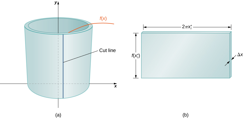
In reality, the outer radius of the shell is greater than the inner radius, and hence the back edge of the plate would be slightly longer than the front edge of the plate. However, we can approximate the flattened shell by a flat plate of height \(f(x^∗_i)\), width \(2 \pi x^∗_i\), and thickness \( \Delta x\) (Figure \( \PageIndex{4} \)(b)). The volume of the shell, then, is approximately the volume of the flat plate. Multiplying the height, width, and depth of the plate, we get
\[V_{\text{shell}} \approx f(x^∗_i)(2 \pi \,x^∗_i)\, \Delta x, \nonumber \]
which is the same formula we had before.
To calculate the volume of the entire solid, we then add the volumes of all the shells and obtain
\[V \approx \sum_{i=1}^n(2 \pi \,x^∗_i f(x^∗_i)\, \Delta x). \nonumber \]
Here we have another Riemann sum, this time for the function \(2 \pi \,x\,f(x).\) Taking the limit as \(n \to \infty \) gives us
\[V=\lim_{n \to \infty }\sum_{i=1}^n(2 \pi \,x^∗_if(x^∗_i)\, \Delta x)=\int ^b_a(2 \pi \,x\,f(x))\,dx. \nonumber \]
This leads to the following rule for the Method of Cylindrical Shells.
Let \(f(x)\) be continuous and nonnegative. Define \(\mathbf{R}\) as the region bounded above by the graph of \(f(x)\), below by the \(x\)-axis, on the left by the line \(x=a\), and on the right by the line \(x=b\). Then the volume of the solid of revolution formed by revolving \(\mathbf{R}\) around the \(y\)-axis is given by
\[V=\int ^b_a(2 \pi \,x\,f(x))\,dx. \nonumber \]
As stated in the previous section, you want to understand how this works rather than memorizing the formula. We will work hard to showcase the thought-process you should go through when using the Method of Cylindrical Shells.
Define \(\mathbf{R}\) as the region bounded above by the graph of \(f(x)=1/x\) and below by the \(x\)-axis over the interval \([1,3]\). Find the volume of the solid of revolution formed by revolving \(\mathbf{R}\) around the \(y\)-axis.
Solution
First we must graph the region \(\mathbf{R}\) and the associated solid of revolution, as shown in Figure \(\PageIndex{5}\). You should also get used to graphing a representative shell (use the CalcPlot3D applet below to visualize this for this example).
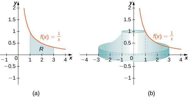
Figure \(\PageIndex{5}\) (c) Visualizing the solid of revolution with CalcPlot3D.
If we had not been told to use the Method of Cylindrical Shells, we would have a choice to make. If you can visualize horizontal slices being rotated about the \( y \)-axis, you would see that the outer radius changes functions at \( y = 1/3 \). This means that you would need two groups of integrals (one for the bottom set of washers, and one for the washers starting at a height of \( y = 1/3 \)). This is highly inefficient.
On the other hand, choosing to make vertical slices and rotating those about the \( y \)-axis shows that the top function of each slice is always \( f(x) = 1/x \) and the bottom function is always \( y = 0 \). Therefore, vertical slicing is a more attractive option.
The volume of the \( i^{\text{th}} \) slice is given in words by
\[ V_i = \left( \text{Circumference of the rotated slice} \right) \left( \text{Height of the rotated slice} \right) \left( \text{Thickness of the rotated slice} \right). \nonumber \]
As per our usual approach, we let \( r(x_i^*) \) be the radius of rotation. We will also let \( h(x_i^*) \) be the height of the slice and naturally select \( \Delta x \) as the thickness. Then our language formula transforms to
\[ \begin{array}{ccccc}
& & \text{Circumference} & \text{Height} & \text{Thickness} \\
V_i & = & 2 \pi r(x_i^*) & h(x_i^*) & \Delta x. \\
\end{array} \nonumber \]
The radius of rotation is the distance between the slice and the axis of rotation (the \( y\)-axis). Since this is a horizontal distance, we measure it as \( x_R - x_L \) (see Measuring Distance from Section 1.1). In this case, \( x_R = x_i^* \) and \( x_L \) is the \( y \)-axis. That is, or \( x_L = 0 \). The height of the slice is a vertical distance, so this should be \( y_T - y_B \) (again, see Measuring Distance from Section 1.1). The top of the slice is \( f(x_i^*) = \frac{1}{x_i^*} \) and the bottom is \( y = 0 \). Putting this altogether, we get
\[ \begin{array}{ccccc}
& & \text{Circumference} & \text{Height} & \text{Thickness} \\
V_i & = & 2 \pi r(x_i^*) & h(x_i^*) & \Delta x \\
& = & 2 \pi x_i^* & \frac{1}{x_i^*} & \Delta x. \\
\end{array} \nonumber \]
Hence, the true volume is
\[ \begin{array}{rcl}
V & = & \displaystyle \int^{x = 3}_{x = 1} \left(2 \pi \,x\left(\dfrac {1}{x}\right)\right)\,dx \\
& = & \displaystyle \int^{x =3}_{x = 1} 2 \pi \,dx \\
& = & 2 \pi \,x\bigg|^{x = 3}_{x = 1} \\
& = & 4 \pi \,\text{units}^3. \\
\end{array} \nonumber\]
Define \(\mathbf{R}\) as the region bounded above by the graph of \(f(x)=x^2\) and below by the \(x\)-axis over the interval \([1,2]\). Find the volume of the solid of revolution formed by revolving \(\mathbf{R}\) around the \(y\)-axis.
- Hint
-
Use the procedure from Example \(\PageIndex{1}\).
- Answer
-
\(\frac{15 \pi }{2} \, \text{units}^3 \)
Define \(\mathbf{R}\) as the region bounded above by the graph of \(f(x)=2x−x^2\) and below by the \(x\)-axis over the interval \([0,2]\). Find the volume of the solid of revolution formed by revolving \(\mathbf{R}\) around the \(y\)-axis.
Solution
First graph the region \(\mathbf{R}\) and the associated solid of revolution, as shown in Figure \(\PageIndex{6}\).

If we chose horizontal slices, we would get washers; however, the outer and inner edges of each washer would be described by the same function. While we could find a way to get the volume of this washer, it would not be the most efficient method. Instead, let's try slicing vertically.
From Figure \( \PageIndex{6} \), we can see that vertical slices would result in cylindrical shells. From Example \( \PageIndex{1} \), we know the volume of the \( i^{\text{th}} \) such shell would be
\[ \begin{array}{ccccc}
& & \text{Circumference} & \text{Height} & \text{Thickness} \\
V_i & = & 2 \pi r(x_i^*) & h(x_i^*) & \Delta x, \\
\end{array} \nonumber \]
where \( r(x_i^*) = x_i^*\) and \( h(x_i^*) = 2x_i^* - (x_i^*)^2 \). Hence,
\[ \begin{array}{ccccc}
& & \text{Circumference} & \text{Height} & \text{Thickness} \\
V_i & = & 2 \pi r(x_i^*) & h(x_i^*) & \Delta x \\
& = & 2 \pi x_i^* & \left( 2x_i^* - (x_i^*)^2 \right) & \Delta x. \\
\end{array} \nonumber \]
Thus,
\[\begin{array}{rcl}
V & = & \displaystyle \int ^2_0(2 \pi \,x(2x−x^2))\,dx \\
& = & 2 \pi \displaystyle \int ^2_0(2x^2−x^3)\,dx \\
& = & 2 \pi \left[\dfrac {2x^3}{3}−\dfrac {x^4}{4}\right]\bigg|^2_0 \\
& = & \dfrac {8 \pi }{3}\,\text{units}^3 \\
\end{array} \nonumber \]
Define \(\mathbf{R}\) as the region bounded above by the graph of \(f(x)=3x−x^2\) and below by the \(x\)-axis over the interval \([0,2]\). Find the volume of the solid of revolution formed by revolving \(\mathbf{R}\) around the \(y\)-axis.
- Hint
-
Use the process from Example \(\PageIndex{2}\).
- Answer
-
\(8 \pi \, \text{units}^3 \)
As with the Disk Method and the Washer Method, we can use the Method of Cylindrical Shells with solids of revolution, revolved around the \(x\)-axis, when we want to integrate with respect to \(y\). The analogous rule for this type of solid is given here. Just to be clear, you should not memorize this formula without truly understanding how to derive it yourself. In fact, commiting this formula to memory is worthless if you truly understand the derivation of the process.
Let \(g(y)\) be continuous and nonnegative. Define \(\mathbf{Q}\) as the region bounded on the right by the graph of \(g(y)\), on the left by the \(y\)-axis, below by the line \(y=c\), and above by the line \(y=d\). Then, the volume of the solid of revolution formed by revolving \(\mathbf{Q}\) around the \(x\)-axis is given by
\[V=\int ^d_c(2 \pi \,y\,g(y))\,dy. \nonumber \]
Define \(\mathbf{Q}\) as the region bounded on the right by the graph of \(g(y)=2\sqrt{y}\) and on the left by the \(y\)-axis for \(y \in [0,4]\). Find the volume of the solid of revolution formed by revolving \(\mathbf{Q}\) around the \(x\)-axis.
Solution
First, we need to graph the region \(\mathbf{Q}\) and the associated solid of revolution, as shown in Figure \(\PageIndex{7}\).

This is a great example where we could easily use either the Washer Method or the Method of Cylindrical Shells. It's advisable to setup both integrals for the practice and to see which one looks easier to evaluate.
VERTICAL SLICES
If we choose vertical slices, we will get washers, which implies the Washer Method. Moreover, each washer will have width \( \Delta x \). This informs us that all of our work should eventually be in terms of \( x \). Let's state the required information first.
\[ r_O(x_i^*) = y_T - y_B = 4 - 0 = 4. \nonumber \]
Finding \( r_I(x_i^*) \) requires us to solve \( x = 2 \sqrt{y} \) for \( y \). This gives \( \frac{x^2}{4} = y \). Therefore,
\[ r_I(x_i^*) = y_T - y_B = \frac{x^2}{4} - 0 = \frac{x^2}{4}. \nonumber \]
The volume of the \( i^{\text{th}} \) slice is
\[ \begin{array}{rcl}
V_i & = & \pi \left[ r_O(x_i^*) \right]^2 \Delta x - \pi \left[ r_I(x_i^*) \right]^2 \Delta x \\
& = & \pi \left( 16 - \dfrac{x^4}{16} \right) \Delta x \\
\end{array} \nonumber \]
Thus,
\[ V = \pi \int_{x = 0}^{x = 4} 16 - \dfrac{x^4}{16} \, dx. \nonumber \]
HORIZONTAL SLICES
If, on the other hand, we decide on horizontal slices, the rotation will result in shells. Hence, we will use the Method of Cylindrical Shells. The thickness of each shell will be \( \Delta y \). This informs us that all of our work should eventually be only in terms of \( y \).
The radius of rotation is \( y_i^* \) and the "height" of each shell is \( x_R - x_L = 2\sqrt{y_i^*} - 0 = 2\sqrt{y_i^*} \). Therefore, the volume of the \( i^{\text{th}} \) slice is
\[ \begin{array}{ccccc}
& & \text{Circumference} & \text{Height} & \text{Thickness} \\
V_i & = & 2 \pi r(y_i^*) & h(y_i^*) & \Delta y \\
& = & 2 \pi y_i^* & \left( 2 \sqrt{y_i^*} \right) & \Delta y. \\
\end{array} \nonumber \]
Then the volume of the solid is given by
\[ V = 4 \pi \int_{y = 0}^{y = 4} y^{3/2} dy. \nonumber \]
You be the judge... which integral looks nicer? While they will both yield the same result, I am choosing the second because... well, it's nicer.
\[ \begin{array}{rcl}
V & = & \displaystyle 4 \pi \int^{y = 4}_{y =0}y^{3/2}\,dy \\
& = & 4 \pi \left[\dfrac {2y^{5/2}}{5}\right]\bigg|^4_0 \\
& = & \dfrac {256 \pi }{5}\, \text{units}^3 \\
\end{array} \nonumber \]
Example \( \PageIndex{3} \) showcases two very important concepts. First, you should not get married to a method. That is, always be willing to try both horizontal and vertical slices. This does not take much time once you get used to things and it can make an impossible problem into a simple one. The second important concept is based on notation. If you look back through Example \( \PageIndex{3} \), you will notice that I wrote the limits of integration as \( x = 0 \) or \( y =0 \), and \( x = 4 \) or \( y = 4 \), accordingly. While the limits didn't change in this example, they often are not the same and writing \( x = \) or \( y = \) will keep your work "honest" and remind you that, yes, you already changed those limits into the proper variable.
Define \(\mathbf{Q}\) as the region bounded on the right by the graph of \(g(y)=3/y\) and on the left by the \(y\)-axis for \(y \in [1,3]\). Find the volume of the solid of revolution formed by revolving \(\mathbf{Q}\) around the \(x\)-axis.
- Hint
-
Use the process from Example \(\PageIndex{3}\).
- Answer
-
\(12 \pi \) units3
Define \(\mathbf{R}\) as the region bounded above by the graph of \(f(x)=x\) and below by the \(x\)-axis over the interval \([1,2]\). Find the volume of the solid of revolution formed by revolving \(\mathbf{R}\) around the line \(x=−1.\)
Solution
First, graph the region \(\mathbf{R}\) and the associated solid of revolution, as shown in Figure \(\PageIndex{8}\).

HORIZONTAL SLICES
If we chose to slice \(\mathbf{R}\) into horizontal slices, we can easily see that we would need two sets of computations - one for the region where the left edge is \( x=1 \) and the right edge is \( x = 2 \), and one for the region where the left edge is \( f(x)=x \) and the right edge is \( x=2 \). This should motivate us to try vertical slices.
VERTICAL SLICES
Slicing the region \(\mathbf{R}\) into vertical slices means that each has a width of \( \Delta x \), and so all of our work needs to be in terms of \( x \). Moreover, a rotation about the vertical line \( x = -1 \) means we are creating shells. The radius of rotation to the \( i^{\text{th}} \) slice is \( x_R - x_L = x_i^* - (-1) = x_i^* + 1 \). The height of the slice is \( h(x_i^*) = y_T - y_B = x_i^* - 0 = x_i^* \). Therefore, the volume of the \( i^{\text{th}} \) slice is
\[ V_i = 2 \pi r(x_i^*) h(x_i^*) \Delta x = 2 \pi (x_i^* + 1) x_i^* \Delta x. \nonumber \]
Thus, the volume of the solid is given by
\[\begin{array}{rcl}
V & = & 2 \pi \displaystyle \int^{x = 2}_{x = 1} x^2+x \, dx \\
& = & 2 \pi \left[\dfrac{x^3}{3}+\dfrac{x^2}{2}\right]\bigg|^2_1 \\
& = & \dfrac{23 \pi }{3} \, \text{units}^3 \\
\end{array} \nonumber\]
Define \(\mathbf{R}\) as the region bounded above by the graph of \(f(x)=x^2\) and below by the \(x\)-axis over the interval \([0,1]\). Find the volume of the solid of revolution formed by revolving \(\mathbf{R}\) around the line \(x=−2\).
- Hint
-
Use the process from Example \(\PageIndex{4}\).
- Answer
-
\(\frac {11 \pi }{6}\) units3
For our final example in this section, let’s look at the volume of a solid of revolution for which the region of revolution is bounded by the graphs of two functions.
Define \(\mathbf{R}\) as the region bounded above by the graph of the function \(f(x)=\sqrt{x}\), below by the graph of the function \(g(x)=1/x\), and on the right by \( x = 4 \). Find the volume of the solid of revolution generated by revolving \(\mathbf{R}\) around the \(y\)-axis.
Solution
First, graph the region \(\mathbf{R}\) and the associated solid of revolution, as shown in Figure \(\PageIndex{9}\). During this process, you will need to find the point of intersection of these two curves, which is \( \left( 1,1 \right) \).

HORIZONTAL OR VERTICAL SLICES?
Since we are rotating about the \( y \)-axis, a quick inspection reveals that horizontal slices yields two separate regions (one below \( y=1 \) and one above \( y = 1 \)), so this is likely not the best choice.
Now that we know to slice vertically, we also gain the knowledge that each slice has width \( \Delta x \). Again, this means all of our eventual work must be in terms of \( x \). Moreover, vertical slices rotated about the \( y \)-axis leads to shells. Hence, we are using the Method of Cylindrical Shells. The radius of rotation for the \( i^{\text{th}} \) shell is \( x_R - x_L = x_i^* - 0 = x_i^* \). The height of this slice is \( h(x_i^*) = y_T - y_B = \sqrt{x_i^*} - \frac{1}{x_i^*} \). Combining this information, we setup the volume of the \( i^{\text{th}} \) slice to be
\[ V_i = 2 \pi r(x_i^*) h(x_i^*) \Delta x = 2 \pi x_i^* \left( \sqrt{x_i^*} - \dfrac{1}{x_i^*} \right) \Delta x. \nonumber \]
Then the volume of the solid is given by
\[\begin{array}{rcl}
V & = & \displaystyle \int^{x = 4}_{x = 1}\left(2 \pi \,x\left(\sqrt{x}−\dfrac {1}{x}\right)\right)\,dx \\
& = & 2 \pi \displaystyle \int^{x = 4}_{x = 1}(x^{3/2}−1)dx \\
& = & 2 \pi \left[\dfrac {2x^{5/2}}{5}−x\right]\bigg|^4_1 \\
& = & \dfrac {94 \pi }{5} \, \text{units}^3. \\
\end{array} \nonumber \]
Define \(\mathbf{R}\) as the region bounded above by the graph of \(f(x)=x\) and below by the graph of \(g(x)=x^2\) over the interval \([0,1]\). Find the volume of the solid of revolution formed by revolving \(\mathbf{R}\) around the \(y\)-axis.
- Hint
-
Hint: Use the process from Example \(\PageIndex{5}\).
- Answer
-
\(\frac { \pi }{6}\) units3
Key Concepts
- The Method of Cylindrical Shells is another method for using a definite integral to calculate the volume of a solid of revolution. This method is sometimes preferable to either the method of disks or the method of washers because we integrate with respect to the other variable. In some cases, one integral is substantially more complicated than the other.
- The geometry of the functions and the difficulty of the integration are the main factors in deciding which integration method to use.
Key Equations
- Method of Cylindrical Shells
\( V=\int ^b_a\left(2 \pi \,x\,f(x)\right)\,dx\)
Glossary
- Method of Cylindrical Shells
- a method of calculating the volume of a solid of revolution by dividing the solid into nested cylindrical shells; this method is different from the methods of disks or washers in that we integrate with respect to the opposite variable