2.1: Separable Equations

Definition 2.1.1

A first order differential equation is separable if it can be written as

\[ h(y)dy=g(x)dx,\]

Rewriting a separable differential equation in the form of Equation 2.1.1 is called separation of variables.

Solving this equation is fairly simple as we need only integrate both sides of the equation with respect to the appropriate variable. Integrating both sides of this equation and combining the constants of integration yields our solution.

Example 2.1.1

Solve the equation

\[{dy\over dx}=x(1+y^2). \nonumber \]

Solution

Separating variables yields

\[{dy\over 1+y^2}=xdx. \nonumber \]

Integrating yields

\[\tan^{-1}y={x^2\over2}+c \nonumber \]

Therefore

\[y=\tan\left({x^2\over2}+c\right). \nonumber \]

Example 2.1.2

1. Solve the equation \[\label{eq:2.2.4} y'=-{x\over y}.\]
2. Solve the initial value problem \[\label{eq:2.2.5} y'=-{x\over y}, \quad y(1)=1.\]
3. Solve the initial value problem \[\label{eq:2.2.6} y'=-{x\over y}, \quad y(1)=-2.\]

Solution a

Separating variables in Equation \ref{eq:2.2.4} yields

\[ydy=-xdx. \nonumber \]

Integrating yields

\[{y^2\over2}=-{x^2\over2}+c, \quad \text{or equivalently} \quad x^2+y^2=2c. \nonumber \]

The last equation shows that \(c\) must be positive if \(y\) is to be a solution of Equation \ref{eq:2.2.4} on an open interval. Therefore we let \(2c=a^2\) (with \(a > 0\)) and rewrite the last equation as

\[\label{eq:2.2.7} x^2+y^2=a^2.\nonumber\]

This equation has two differentiable solutions for \(y\) in terms of \(x\):

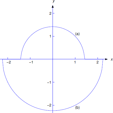
\[\label{eq:2.2.8} y=\phantom{-} \sqrt{a^2-x^2}, \quad -a < x < a,\]

and

\[\label{eq:2.2.9} y= - \sqrt{a^2-x^2}, \quad -a < x < a.\]

The solution curves defined by Equation \ref{eq:2.2.8} are semicircles above the \(x\)-axis and those defined by Equation \ref{eq:2.2.9} are semicircles below the \(x\)-axis.

Solution b

The solution of Equation \ref{eq:2.2.5} is positive when \(x=1\); hence, it is of the form Equation \ref{eq:2.2.8}. Substituting \(x=1\) and \(y=1\) into Equation \ref{eq:2.2.8} to satisfy the initial condition yields \(a^2=2\); hence, the solution of Equation \ref{eq:2.2.5} is

\[y=\sqrt{2-x^2}, \quad - \sqrt{2}< x < \sqrt{2}. \nonumber \]

Solution c

The solution of Equation \ref{eq:2.2.6} is negative when \(x=1\) and is therefore of the form Equation \ref{eq:2.2.9}. Substituting \(x=1\) and \(y=-2\) into Equation \ref{eq:2.2.9} to satisfy the initial condition yields \(a^2=5\). Hence, the solution of Equation \ref{eq:2.2.6} is

\[y=- \sqrt{5-x^2}, \quad -\sqrt{5} < x < \sqrt{5}. \nonumber \]

Figure 2.1.1 : (b) \(y=\sqrt{2-x^2}, - \sqrt{2}< x < \sqrt{2} \nonumber \); \({}\) (c) \(y=- \sqrt{5-x^2}, -\sqrt{5} < x < \sqrt{5}. \nonumber \)

Implicit Solutions of Separable Equations

In Examples 2.1.1 and 2.1.2 we were able to solve the equation for the dependent variable \(y\) to obtain explicit formulas for solutions of the given separable differential equations. As we’ll see in the next example, this isn’t always possible. In this situation we must broaden our definition of a solution of a separable equation. The next theorem provides the basis for this modification. We omit the proof, which requires a result from advanced calculus.

Theorem 2.1.1 Implicit Function Theorem

Suppose \(g=g(x)\) is continuous on \((a,b)\) and \(h=h(y)\) is continuous on \((c,d).\) Let \(G\) be an antiderivative of \(g\) on \((a,b)\) and let \(H\) be an antiderivative of \(h\) on \((c,d).\) Let \(x_0\) be an arbitrary point in \((a,b),\) let \(y_0\) be a point in \((c,d)\) such that \(h(y_0)\ne0,\) and define

\[\label{eq:2.2.10} c=H(y_0)-G(x_0).\]

Then there’s a function \(y=y(x)\) defined on some open interval \((a_1,b_1),\) where \(a\le a_1<x_0<b_1\le b\), such that \(y(x_0)=y_0\) and

\[\label{eq:2.2.11} H(y)=G(x)+c\]

for \(a_1<x<b_1\). Therefore \(y\) is a solution of the initial value problem

\[\label{eq:2.2.12} h(y)dy=g(x)dx,\quad y(x_0)=y_0.\]

It’s convenient to say that Equation \ref{eq:2.2.11} with \(c\) arbitrary is an implicit solution of \(h(y)dy=g(x)dx\). Curves defined by Equation \ref{eq:2.2.11} are integral curves of \(h(y)dy=g(x)dx\). If \(c\) satisfies Equation \ref{eq:2.2.10}, we’ll say that Equation \ref{eq:2.2.11} is an implicit solution of the initial value problem Equation \ref{eq:2.2.12}. However, keep these points in mind:

• For some choices of \(c\) there may not be any differentiable functions \(y\) that satisfy Equation \ref{eq:2.2.11}.
• The function \(y\) in Equation \ref{eq:2.2.11} (not Equation \ref{eq:2.2.11} itself) is a solution of \(h(y)dy=g(x)dx\).

Example 2.1.3

1. Find implicit solutions of \[\label{eq:2.2.13} y'={2x+1\over5y^4+1}.\]
2. Find an implicit solution of \[\label{eq:2.2.14} y'={2x+1\over5y^4+1},\quad y(2)=1.\]

Solution a

Separating variables yields

\[(5y^4+1)dy=(2x+1)dx. \nonumber \]

Integrating yields the implicit solution

\[\label{eq:2.2.15} y^5+y=x^2+x+ c. \]

of Equation \ref{eq:2.2.13}.

Solution b

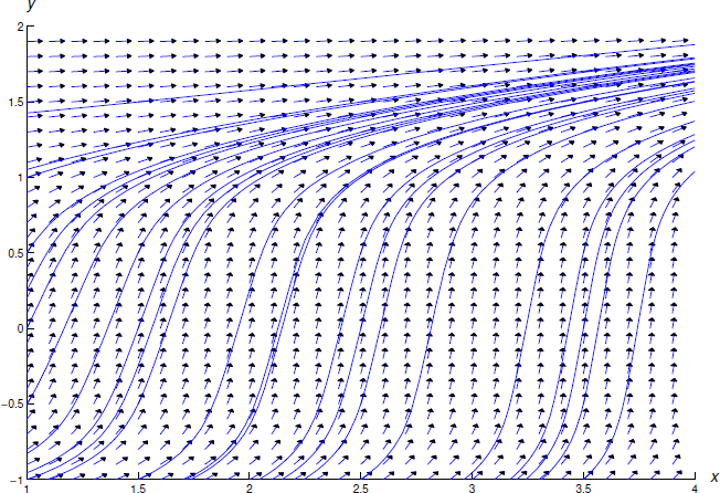
Imposing the initial condition \(y(2)=1\) in Equation \ref{eq:2.2.15} yields \(1+1=4+2+c\), so \(c=-4\). Therefore

\[y^5+y=x^2+x-4 \nonumber \]

is an implicit solution of the initial value problem Equation \ref{eq:2.2.14}. Although more than one differentiable function \(y=y(x)\) satisfies Equation \ref{eq:2.2.13} near \(x=1\), it can be shown that there is only one such function that satisfies the initial condition \(y(1)=2\). Figure 2.1.2 shows a direction field and some integral curves for Equation \ref{eq:2.2.13}.

Figure 2.1.2 : A direction field and integral curves for \(y'= {\frac{2x+1}{5y^{4}+1}}\)

Singular Solutions of Separable Equations

An equation of the form

\[y'=g(x)p(y) \nonumber \]

is separable, since it can be rewritten as

\[{1\over p(y)}dy=g(x)dx. \nonumber \]

However, the division by \(p(y)\) is not legitimate if \(p(y)=0\) for some values of \(y\). The next two examples show how to deal with this problem.

Example 2.1.4

Find all solutions of

\[\label{eq:2.2.16} y'=2xy^2.\]

Solution

Here we must divide by \(p(y)=y^2\) to separate variables. This isn’t legitimate if \(y\) is a solution of Equation \ref{eq:2.2.16} that equals zero for some value of \(x\). One such solution can be found by inspection: \(y \equiv 0\). Now suppose \(y\) is a solution of Equation \ref{eq:2.2.16} that isn’t identically zero. Since \(y\) is continuous there must be an interval on which \(y\) is never zero. Since division by \(y^2\) is legitimate for \(x\) in this interval, we can separate variables in Equation \ref{eq:2.2.16} to obtain

\[{dy\over y^2}=2xdx. \nonumber \]

Integrating this yields

\[-{1\over y}=x^2+c, \nonumber \]

which is equivalent to

\[\label{eq:2.2.17} y=-{1\over x^2+c}.\]

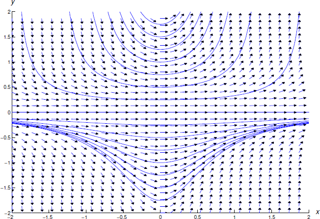
We’ve now shown that if \(y\) is a solution of Equation \ref{eq:2.2.16} that is not identically zero, then \(y\) must be of the form Equation \ref{eq:2.2.17}. By substituting Equation \ref{eq:2.2.17} into Equation \ref{eq:2.2.16}, you can verify that Equation \ref{eq:2.2.17} is a solution of Equation \ref{eq:2.2.16}. Thus, solutions of Equation \ref{eq:2.2.16} are \(y\equiv0\) and the functions of the form Equation \ref{eq:2.2.17}. Note that the solution \(y\equiv0\) isn’t of the form Equation \ref{eq:2.2.17} for any value of \(c\). Because of this, \(y\equiv0\) is called a singular solution of \ref{eq:2.2.16} because it cannot be obtained from the family of solutions \ref{eq:2.2.17}.

Figure 2.1.3 shows a direction field and some integral curves for Equation \ref{eq:2.2.16}

Figure 2.1.3 : A direction field and integral curves for \(y'=2xy^{2}\)

Example 2.1.5

Find all solutions of

\[\label{eq:2.2.18} y'={1\over2}x(1-y^2). \]

Here we must divide by \(p(y)=1-y^2\) to separate variables. This isn’t legitimate if \(y\) is a solution of Equation \ref{eq:2.2.18} that equals \(\pm1\) for some value of \(x\). Two such solutions can be found by inspection: \(y \equiv 1\) and \(y\equiv-1\). Now suppose \(y\) is a solution of Equation \ref{eq:2.2.18} such that \(1-y^2\) isn’t identically zero. Since \(1-y^2\) is continuous there must be an interval on which \(1-y^2\) is never zero. Since division by \(1-y^2\) is legitimate for \(x\) in this interval, we can separate variables in Equation \ref{eq:2.2.18} to obtain

\[{2dy\over y^2-1}=-xdx. \nonumber \]

A partial fraction expansion on the left yields

\[\left[{1\over y-1}-{1\over y+1}\right]y'=-x, \nonumber \]

and integrating yields

\[\ln\left|{y-1\over y+1}\right|=-{x^2\over2}+k; \nonumber \]

hence,

\[\left|{y-1\over y+1}\right|=e^ke^{-x^2/2}. \nonumber \]

Since \(y(x)\ne\pm1\) for \(x\) on the interval under discussion, the quantity \((y-1)/(y+1)\) cannot change sign in this interval. Therefore we can rewrite the last equation as

\[{y-1\over y+1}=ce^{-x^2/2}, \nonumber \]

where \(c=\pm e^k\), depending upon the sign of \((y-1)/(y+1)\) on the interval. Solving for \(y\) yields

\[\label{eq:2.2.19} y={1+ce^{-x^2/2}\over 1-ce^{-x^2/2}}. \]

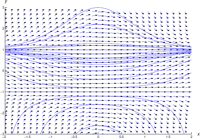
We’ve now shown that if \(y\) is a solution of Equation \ref{eq:2.2.18} that is not identically equal to \(\pm1\), then \(y\) must be as in Equation \ref{eq:2.2.19}. By substituting Equation \ref{eq:2.2.19} into Equation \ref{eq:2.2.18} you can verify that Equation \ref{eq:2.2.19} is a solution of Equation \ref{eq:2.2.18}. Thus, the solutions of Equation \ref{eq:2.2.18} are \(y\equiv1\), \(y\equiv-1\) and the functions of the form Equation \ref{eq:2.2.19}. Note that the constant solution \(y \equiv 1\) can be obtained from this formula by taking \(c=0\); however, the other constant solution, \(y \equiv -1\), cannot be obtained in this way. Thus, \(y \equiv 1\) comes from the family of solutions and \(y \equiv -1\) is a singular solution.

Figure 2.1.4 shows a direction field and some integrals for Equation \ref{eq:2.2.18}.

Figure 2.1.4 : A direction field and integral curves for \(y'= {\frac{x(1-y^2)}{2}}\)

Example 2.1.6

Solve the initial value problem

\[y'=2xy^2, \quad y(0)=y_0 \nonumber \]

and determine the interval of validity of the solution.

Solution

First suppose \(y_0\ne0\). From Example 2.1.4 , we know that \(y\) must be of the form

\[\label{eq:2.2.20} y=-{1\over x^2+c}.\]

Imposing the initial condition shows that \(c=-1/y_0\). Substituting this into Equation \ref{eq:2.2.20} and rearranging terms yields the solution

\[y= {y_0\over 1-y_0x^2}. \nonumber \]

This is also the solution if \(y_0=0\). If \(y_0<0\), the denominator isn’t zero for any value of \(x\), so the the solution is valid on \((-\infty,\infty)\). If \(y_0>0\), the solution is valid only on \((-1/\sqrt{y_0},1/\sqrt{y_0})\) (recall that the interval must always include \(x_0\); in this case 0).