
5.4: Nonhomogeneous Linear Equations
- Page ID
- 103503

\( \newcommand{\vecs}[1]{\overset { \scriptstyle \rightharpoonup} {\mathbf{#1}} } \)
\( \newcommand{\vecd}[1]{\overset{-\!-\!\rightharpoonup}{\vphantom{a}\smash {#1}}} \)
\( \newcommand{\id}{\mathrm{id}}\) \( \newcommand{\Span}{\mathrm{span}}\)
( \newcommand{\kernel}{\mathrm{null}\,}\) \( \newcommand{\range}{\mathrm{range}\,}\)
\( \newcommand{\RealPart}{\mathrm{Re}}\) \( \newcommand{\ImaginaryPart}{\mathrm{Im}}\)
\( \newcommand{\Argument}{\mathrm{Arg}}\) \( \newcommand{\norm}[1]{\| #1 \|}\)
\( \newcommand{\inner}[2]{\langle #1, #2 \rangle}\)
\( \newcommand{\Span}{\mathrm{span}}\)
\( \newcommand{\id}{\mathrm{id}}\)
\( \newcommand{\Span}{\mathrm{span}}\)
\( \newcommand{\kernel}{\mathrm{null}\,}\)
\( \newcommand{\range}{\mathrm{range}\,}\)
\( \newcommand{\RealPart}{\mathrm{Re}}\)
\( \newcommand{\ImaginaryPart}{\mathrm{Im}}\)
\( \newcommand{\Argument}{\mathrm{Arg}}\)
\( \newcommand{\norm}[1]{\| #1 \|}\)
\( \newcommand{\inner}[2]{\langle #1, #2 \rangle}\)
\( \newcommand{\Span}{\mathrm{span}}\) \( \newcommand{\AA}{\unicode[.8,0]{x212B}}\)
\( \newcommand{\vectorA}[1]{\vec{#1}} % arrow\)
\( \newcommand{\vectorAt}[1]{\vec{\text{#1}}} % arrow\)
\( \newcommand{\vectorB}[1]{\overset { \scriptstyle \rightharpoonup} {\mathbf{#1}} } \)
\( \newcommand{\vectorC}[1]{\textbf{#1}} \)
\( \newcommand{\vectorD}[1]{\overrightarrow{#1}} \)
\( \newcommand{\vectorDt}[1]{\overrightarrow{\text{#1}}} \)
\( \newcommand{\vectE}[1]{\overset{-\!-\!\rightharpoonup}{\vphantom{a}\smash{\mathbf {#1}}}} \)
\( \newcommand{\vecs}[1]{\overset { \scriptstyle \rightharpoonup} {\mathbf{#1}} } \)
\( \newcommand{\vecd}[1]{\overset{-\!-\!\rightharpoonup}{\vphantom{a}\smash {#1}}} \)
We’ll now consider the nonhomogeneous linear second order equation
\[\label{eq:5.3.1} y''+p(x)y'+q(x)y=f(x),\]
where the forcing function \(f\) isn’t identically zero. The next theorem, an extension of Theorem 5.1.1, gives sufficient conditions for existence and uniqueness of solutions of initial value problems for Equation \ref{eq:5.3.1}. We omit the proof, which is beyond the scope of this book.
Suppose \(p,\) \(q,\) and \(f\) are continuous on an open interval \((a,b),\) let \(x_0\) be any point in \((a,b),\) and let \(k_0\) and \(k_1\) be arbitrary real numbers\(.\) Then the initial value problem
\[y''+p(x)y'+q(x)y=f(x), \quad y(x_0)=k_0,\quad y'(x_0)=k_1\nonumber \]
has a unique solution on \((a,b).\)
To find the general solution of Equation \ref{eq:5.3.1} on an interval \((a,b)\) where \(p\), \(q\), and \(f\) are continuous, it is necessary to find the general solution of the associated homogeneous equation
\[\label{eq:5.3.2} y''+p(x)y'+q(x)y=0\]
on \((a,b)\). We call Equation \ref{eq:5.3.2} the homogeneous equation for Equation \ref{eq:5.3.1}.
The next theorem shows how to find the general solution of Equation \ref{eq:5.3.1} if we know one solution \(y_p\) of Equation \ref{eq:5.3.1} and a fundamental set of solutions of Equation \ref{eq:5.3.2}. We call \(y_p\) a particular solution of Equation \ref{eq:5.3.1}; it can be any solution that we can find, one way or another.
Suppose \(p,\) \(q,\) and \(f\) are continuous on \((a,b).\) Let \(y_p\) be a particular solution of
\[\label{eq:5.3.3} y''+p(x)y'+q(x)y=f(x)\]
on \((a,b)\), and let \(\{y_1,y_2\}\) be a fundamental set of solutions of the homogeneous equation
\[\label{eq:5.3.4} y''+p(x)y'+q(x)y=0\]
on \((a,b)\). Then \(y\) is a solution of \(\eqref{eq:5.3.3}\) on \((a,b)\) if and only if
\[\label{eq:5.3.5} y=y_p+c_1y_1+c_2y_2,\]
where \(c_1\) and \(c_2\) are constants
We first show that \(y\) in Equation \ref{eq:5.3.5} is a solution of Equation \ref{eq:5.3.3} for any choice of the constants \(c_1\) and \(c_2\). Differentiating Equation \ref{eq:5.3.5} twice yields
\[y'=y_p'+c_1y_1'+c_2y_2' \quad \text{and} \quad y''=y_p''+ c_1y_1''+c_2y_2'', \nonumber\]
so
\[\begin{align*} y''+p(x)y'+q(x)y&=(y_p''+c_1y_1''+c_2y_2'') +p(x)(y_p'+c_1y_1'+c_2y_2') +q(x)(y_p+c_1y_1+c_2y_2)\\ &=(y_p''+p(x)y_p'+q(x)y_p)+c_1(y_1''+p(x)y_1'+q(x)y_1) +c_2(y_2''+p(x)y_2'+q(x)y_2)\\ &= f+c_1\cdot0+c_2\cdot0=f,\end{align*}\]
since \(y_p\) satisfies Equation \ref{eq:5.3.3} and \(y_1\) and \(y_2\) satisfy Equation \ref{eq:5.3.4}.
Now we’ll show that every solution of Equation \ref{eq:5.3.3} has the form Equation \ref{eq:5.3.5} for some choice of the constants \(c_1\) and \(c_2\). Suppose \(y\) is a solution of Equation \ref{eq:5.3.3}. We’ll show that \(y-y_p\) is a solution of Equation \ref{eq:5.3.4}, and therefore of the form \(y-y_p=c_1y_1+c_2y_2\), which implies Equation \ref{eq:5.3.5}. To see this, we compute
\[\begin{align*} (y-y_p)''+p(x)(y-y_p)'+q(x)(y-y_p)&=(y''-y_p'')+p(x)(y'-y_p') +q(x)(y-y_p)\\ &=(y''+p(x)y'+q(x)y) -(y_p''+p(x)y_p'+q(x)y_p)\\ &=f(x)-f(x)=0,\end{align*}\]
since \(y\) and \(y_p\) both satisfy Equation \ref{eq:5.3.3}.
We say that Equation \ref{eq:5.3.5} is the general solution of \(\eqref{eq:5.3.3}\) on \((a,b)\).
If \(P_0\), \(P_1\), and \(F\) are continuous and \(P_0\) has no zeros on \((a,b)\), then Theorem 5.4.2 implies that the general solution of
\[\label{eq:5.3.6} P_0(x)y''+P_1(x)y'+P_2(x)y=F(x)\]
on \((a,b)\) is \(y=y_p+c_1y_1+c_2y_2\), where \(y_p\) is a particular solution of Equation \ref{eq:5.3.6} on \((a,b)\) and \(\{y_1,y_2\}\) is a fundamental set of solutions of
\[P_0(x)y''+P_1(x)y'+P_2(x)y=0\nonumber\]
on \((a,b)\). To see this, we rewrite Equation \ref{eq:5.3.6} as
\[y''+{P_1(x)\over P_0(x)}y'+{P_2(x)\over P_0(x)}y={F(x)\over P_0(x)}\nonumber\]
and apply Theorem 5.4.2 with \(p=P_1/P_0\), \(q=P_2/P_0\), and \(f=F/P_0\).
To avoid awkward wording in examples and exercises, we will not specify the interval \((a,b)\) when we ask for the general solution of a specific linear second order equation, or for a fundamental set of solutions of a homogeneous linear second order equation. Let’s agree that this always means that we want the general solution (or a fundamental set of solutions, as the case may be) on every open interval on which \(p\), \(q\), and \(f\) are continuous if the equation is of the form Equation \ref{eq:5.3.3}, or on which \(P_0\), \(P_1\), \(P_2\), and \(F\) are continuous and \(P_0\) has no zeros, if the equation is of the form Equation \ref{eq:5.3.6}. We leave it to you to identify these intervals in specific examples and exercises.
For completeness, we point out that if \(P_0\), \(P_1\), \(P_2\), and \(F\) are all continuous on an open interval \((a,b)\), but \(P_0\) does have a zero in \((a,b)\), then Equation \ref{eq:5.3.6} may fail to have a general solution on \((a,b)\) in the sense just defined.
The next three examples illustrate concepts that we’ll develop later in this chapter. As in section 5.1, you shouldn’t be concerned with how to find the given particular solutions of the equations in these examples. This will be explained in later sections. In this section we limit ourselves to applications of Theorem 5.4.2 where we are given the particular solution.
- Find the general solution of \[\label{eq:5.3.7} y''+y=1.\]
- Solve the initial value problem \[\label{eq:5.3.8} y''+y=1, \quad y(0)=2,\quad y'(0)=7.\]
Solution
a. We can apply Theorem 5.4.2 with \((a,b)= (-\infty,\infty)\), since the functions \(p\equiv0\), \(q\equiv1\), and \(f\equiv1\) in Equation \ref{eq:5.3.7} are continuous on \((-\infty,\infty)\). By inspection we see that \(y_p\equiv1\) is a particular solution of Equation \ref{eq:5.3.7}. Since \(y_1=\cos x\) and \(y_2=\sin x\) form a fundamental set of solutions of the complementary equation \(y''+y=0\), the general solution of Equation \ref{eq:5.3.7} is
\[\label{eq:5.3.9} y=c_1\cos x + c_2\sin x+1.\]
b. Imposing the initial condition \(y(0)=2\) in Equation \ref{eq:5.3.9} yields \(2=1+c_1\), so \(c_1=1\). Differentiating Equation \ref{eq:5.3.9} yields
\[y'=-c_1\sin x+c_2\cos x.\nonumber\]
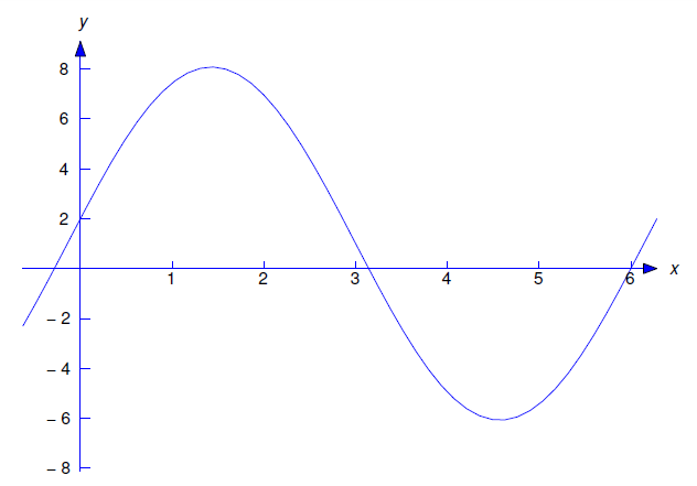
Imposing the initial condition \(y'(0)=7\) here yields \(c_2=7\), so the solution of Equation \ref{eq:5.3.8} is
\[y=\cos x+7\sin x+1.\nonumber\]
Figure 5.4.1 is a graph of this function.
- Find the general solution of \[\label{eq:5.3.10} y''-2y'+y=-3-x+x^2.\]
- Solve the initial value problem \[\label{eq:5.3.11} y''-2y'+y=-3-x+x^2, \quad y(0)=-2,\quad y'(0)=1.\]
Solution
a. The characteristic equation of the homogeneous equation
\[y''-2y'+y=0 \nonumber\]
is \(r^2-2r+1=(r-1)^2\), so \(y_1=e^x\) and \(y_2=xe^x\) form a fundamental set of solutions of the homogeneous equation.
\(y_p=1+3x+x^2\) is a particular solution of Equation \ref{eq:5.3.10} (verify) and Theorem 5.4.2 implies that
\[\label{eq:5.3.12} y=1+3x+x^2+e^x(c_1+c_2x)\]
is the general solution of Equation \ref{eq:5.3.10}.
b. Imposing the initial condition \(y(0)=-2\) in Equation \ref{eq:5.3.12} yields \(-2=1+c_1\), so \(c_1=-3\). Differentiating Equation \ref{eq:5.3.12} yields
\[y'=3+2x+e^x(c_1+c_2x)+c_2e^x,\nonumber\]
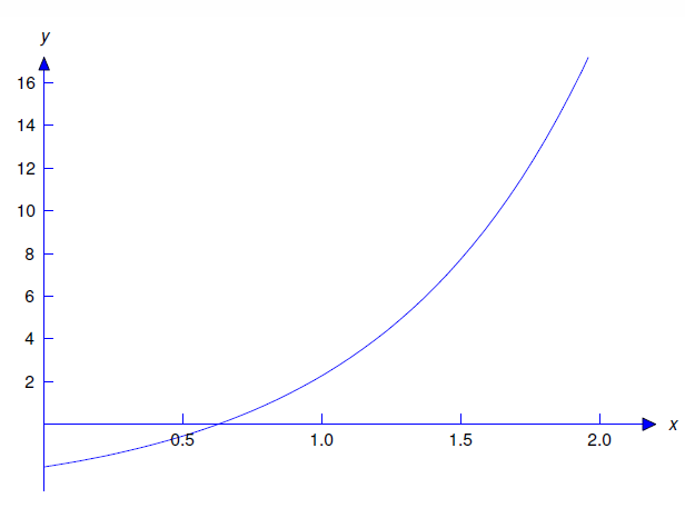
and imposing the initial condition \(y'(0)=1\) here yields \(1=3+c_1+c_2\), so \(c_2=1\). Therefore the solution of Equation \ref{eq:5.3.11} is
\[y=1+3x+x^2-e^x(3-x). \nonumber\]
Figure 5.4.2 is a graph of this solution.
Find the general solution of
\[\label{eq:5.3.13} x^2y''+xy'-4y=2x^4\]
on \((-\infty,0)\) and \((0,\infty)\).
Solution
In Example 5.1.2, we verified that \(y_1=x^2\) and \(y_2=1/x^2\) form a fundamental set of solutions of the homogeneous equation
\[x^2y''+xy'-4y=0 \nonumber\]
on \((-\infty,0)\) and \((0,\infty)\).
\(y_p=x^4/6\) is a particular solution of Equation \ref{eq:5.3.13} (verify) on \((-\infty,\infty)\). Theorem 5.4.2 implies that the general solution of Equation \ref{eq:5.3.13} on \((-\infty,0)\) and \((0,\infty)\) is
\[y={x^4\over6}+c_1x^2+{c_2\over x^2}. \nonumber\]
The Principle of Superposition
The next theorem enables us to break a nonhomogeneous equation into simpler parts, find a particular solution for each part, and then combine their solutions to obtain a particular solution of the original problem.
Suppose \(y_{p_1}\) is a particular solution of
\[y''+p(x)y'+q(x)y=f_1(x) \nonumber\]
on \((a,b)\) and \(y_{p_2}\) is a particular solution of
\[y''+p(x)y'+q(x)y=f_2(x) \nonumber\]
on \((a,b)\). Then
\[y_p=y_{p_1}+y_{p_2} \nonumber\]
is a particular solution of
\[y''+p(x)y'+q(x)y=f_1(x)+f_2(x) \nonumber\]
on \((a,b)\)
If \(y_p=y_{p_1}+y_{p_2}\) then
\[\begin{align*} y_p''+p(x)y_p'+q(x)y_p&=(y_{p_1}+y_{p_2})''+p(x)(y_{p_1}+y_{p_2})' +q(x)(y_{p_1}+y_{p_2})\\ &=\left(y_{p_1}''+p(x)y_{p_1}'+q(x)y_{p_1}\right) +\left(y_{p_2}''+p(x)y_{p_2}'+q(x)y_{p_2}\right)\\ &=f_1(x)+f_2(x). \end{align*}\]
It’s easy to generalize Theorem 5.4.3 to the equation
\[\label{eq:5.3.14} y''+p(x)y'+q(x)y=f(x)\]
where
\[f=f_1+f_2+\cdots+f_k; \nonumber\]
thus, if \(y_{p_i}\) is a particular solution of
\[y''+p(x)y'+q(x)y=f_i(x) \nonumber\]
on \((a,b)\) for \(i=1\), \(2\), …, \(k\), then \(y_p=y_{p_1}+y_{p_2}+\cdots+y_{p_k}\) is a particular solution of Equation \ref{eq:5.3.14} on \((a,b)\).
The function \(y_{p_1}=x^4/15\) is a particular solution of
\[\label{eq:5.3.15} x^2y''+4xy'+2y=2x^4\]
on \((-\infty,\infty)\) and \(y_{p_2}=x^2/3\) is a particular solution of\[\label{eq:5.3.16} x^2y''+4xy'+2y=4x^2\]
on \((-\infty,\infty)\). Use the principle of superposition to find a particular solution of\[\label{eq:5.3.17} x^2y''+4xy'+2y=2x^4+4x^2\]
on \((-\infty,\infty)\).
Solution
The right side \(F(x)=2x^4+4x^2\) in Equation \ref{eq:5.3.17} is the sum of the right sides
\[F_1(x)=2x^4\quad \text{and} \quad F_2(x)=4x^2. \nonumber\]
in Equation \ref{eq:5.3.15} and Equation \ref{eq:5.3.16}. Therefore the principle of superposition implies that\[y_p=y_{p_1}+y_{p_2}={x^4\over15}+{x^2\over3} \nonumber\]
is a particular solution of Equation \ref{eq:5.3.17}.