9.2: The Standard Normal Distribution

Learning Objectives

• Identify the characteristics of a standard normal distribution.
• Compute probabilities using a standard normal distribution.

While it is convenient to estimate areas under a normal curve using the Empirical Rule, we often need more precise methods to calculate these areas. Luckily, we can use formulas or technology to help us with the calculations. All normal distributions have the same basic shape, and therefore, rescaling and re-centering can be implemented to change any normal distribution to one with a mean of 0 and a standard deviation of 1. This configuration is referred to as a standard normal distribution. In a standard normal distribution, the variable along the horizontal axis is the z-score.

Standard Normal Distribution

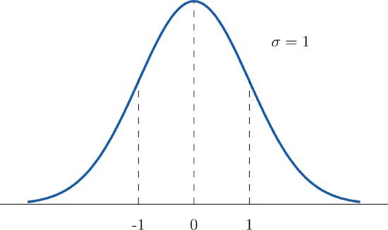
A standard normal distribution is a normal distribution with mean \(\mu =0\) and standard deviation \(\sigma =1\). It is denoted by the letter \(Z\).

The curve for a standard normal distribution is shown below. Note the mean is 0 and the standard deviation is 1.

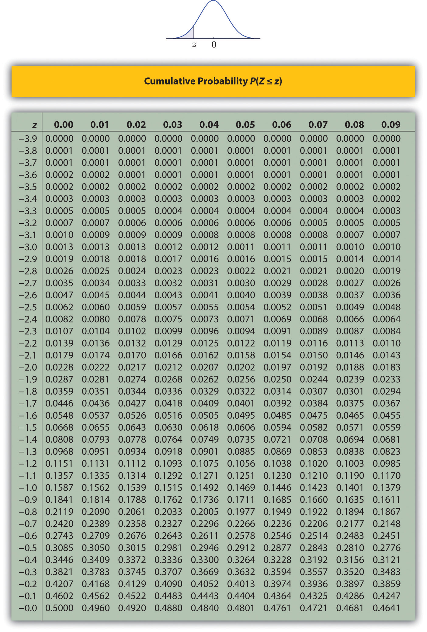
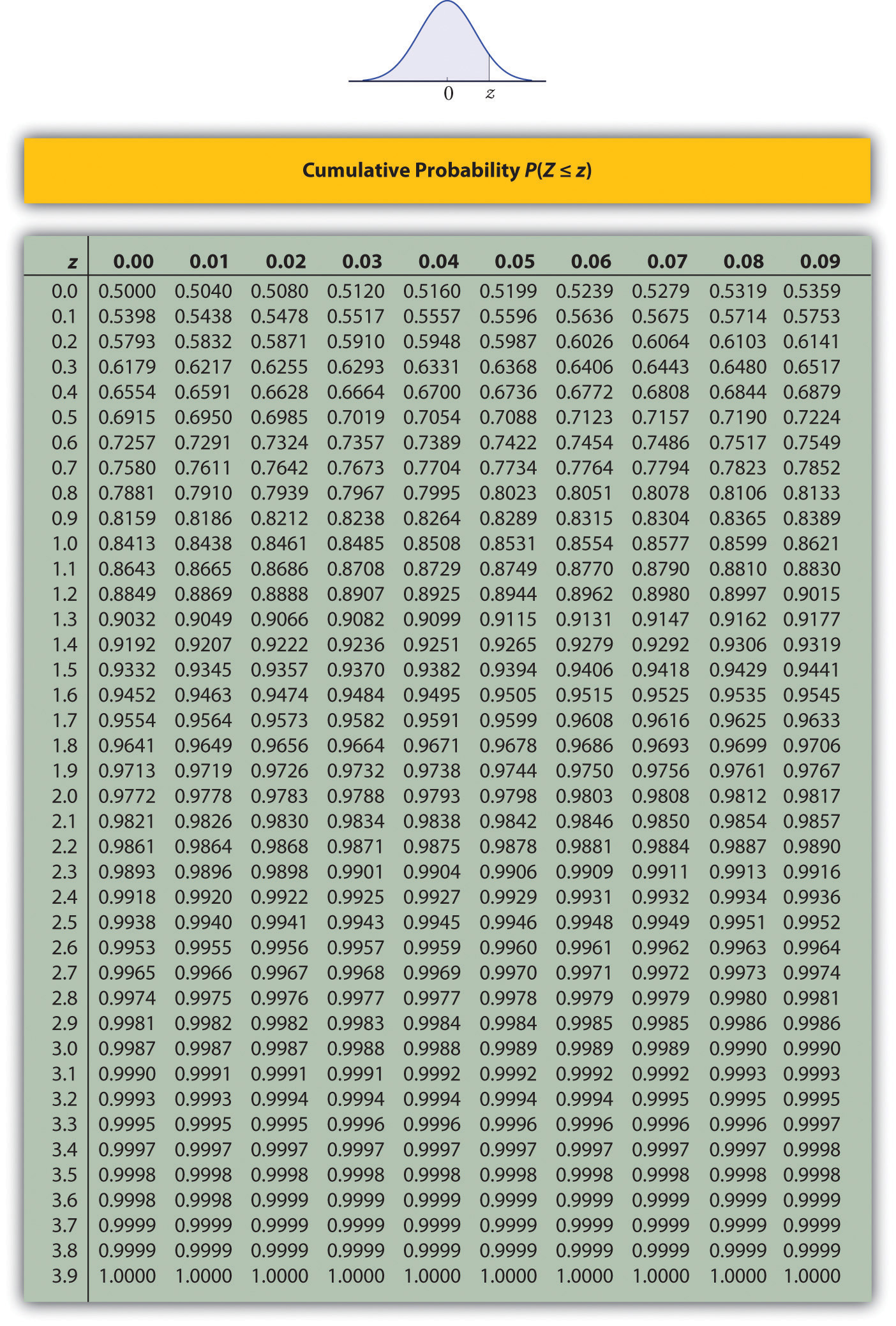
Since areas under normal curves correspond to the probability of an event occurring, a special normal distribution table is used to calculate the probabilities. To find probabilities for \(Z\), we will read probabilities out of the tables below. The tables contain cumulative probabilities; their entries are probabilities of the form \(P(Z \leq z)\). This means the probability in the table is the probability or area to the left of the value of \(z\). Probabilities for negative values of \(z\) are found in the first page of the table while probabilities for positive values of \(z\) are found on the second page. The table is also available online here in section 6. The use of the tables will be explained by the following series of examples.

Example \(\PageIndex{1}\)

Find the probabilities indicated, where \(Z\) denotes a standard normal distribution.

1. The probability of selecting a value less than or equal to \(z = 1.48\), or \(P(Z \leq 1.48)\).
2. The probability of selecting a value less than or equal to \(z = -0.25\), or \(P(Z \leq -0.25)\).

Solution:

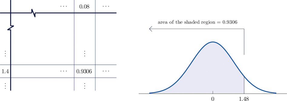
1. It is first helpful to draw the standard normal curve, label the mean, label the given \(z\)-value, and shade the area of the probability desired. For this problem, we would draw the standard normal curve and label 0 on the \(x\)-axis at the peak. Then we would estimate where \(z = 1.48\) would be to the right of the mean at 0. Since we are finding the probability of selecting a value less than or equal to \(z\), we would shade the area to the left.
   
   The figure below shows how this probability is read directly from the table without any computation required. We need to look at the second page of the table since the \(z\)-value is positive. The digits in the ones and tenths places of \(1.48\), namely \(1.4\), are used to select the appropriate row of the table; the hundredths part of \(1.48\), namely \(0.08\), is used to select the appropriate column of the table. The 4-decimal place number in the interior of the table that lies in the intersection of the row and column selected, \(0.9306\), is the probability sought since we are looking for the probability to the left of \(z = 1.48\):

\[P(Z \leq 1.48)=0.9306 \nonumber\]

2. The minus sign in \(z = -0.25\) makes no difference in the procedure; the table is used in exactly the same way as in part (a): the probability sought is the number that is in the intersection of the row with heading \(-0.2\) and the column with heading \(0.05\), the number \(0.4013\). Thus \(P(Z \leq -0.25)=0.4013\).

Example \(\PageIndex{2}\)

Find the probabilities indicated.

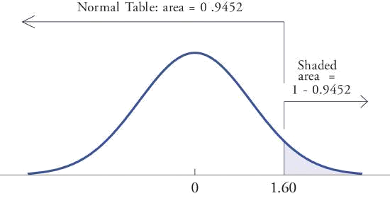
1. The probability of selecting a value greater than \(z = 1.60\), or \(P(Z> 1.60)\).
2. The probability of selecting a value greater than \(z = -1.02\), or \(P(Z> -1.02)\).

Solution:

1. Because the events \(Z> 1.60\) and \(Z\leq 1.60\) are complements, the probability rule for the complement of an event implies that \[P(Z> 1.60)=1-P(Z\leq 1.60)\] Since inclusion of the endpoint makes no difference for the standard normal curve \(Z\), \(P(Z\leq 1.60)=P(Z< 1.60)\), which we know how to find from the table. The number in the row with heading \(1.6\) and in the column with heading \(0.00\) is \(0.9452\). Thus \(P(Z< 1.60)=0.9452\) so \[P(Z> 1.60)=1-P(Z\leq 1.60)=1-0.9452=0.0548\] The figure below illustrates the sketch of the probability desired. Since the total area under the curve is \(1\) and the area of the region to the left of \(1.60\) is (from the table) \(0.9452\), the area of the region to the right of \(1.60\) must be \(1-0.9452=0.0548\). Thus, (P(Z> 1.60)= 0.0548\).

2. The minus sign in \(-1.02\) makes no difference in the procedure; the table is used in exactly the same way as in part (a). The number in the intersection of the row with heading \(-1.0\) and the column with heading \(0.02\) is \(0.1539\). This means that \(P(Z<-1.02)=P(Z\leq -1.02)=0.1539\). Hence \(P(Z>-1.02)=1-P(Z\leq -1.02)=1-0.1539=0.8461\).

Example \(\PageIndex{3}\)

Find the probabilities indicated.

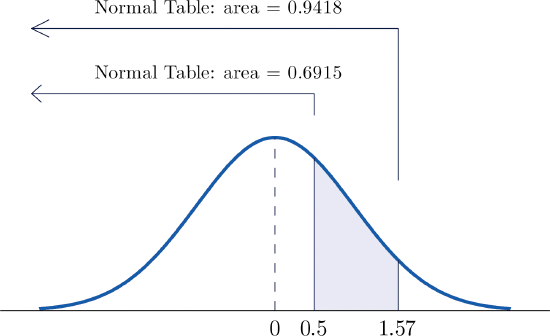
1. The probability of selecting a value between \(z = 0.5\) and \(z = 1.57\) or \(P(0.5<Z<1.57)\).
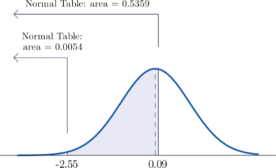
2. The probability of selecting a value between \(z = -2.55\) and \(z = 0.09\) or \(P(-2.55<Z<0.09)\).

Solution:

1. The figure below illustrates the ideas involved for intervals of this type. First look up the areas in the table that correspond to the numbers \(z = 0.5\) (which we think of as \(z = 0.50\) to use the table) and \(z = 1.57\). We obtain \(0.6915\) and \(0.9418\), respectively. From the figure it is apparent that we must take the difference of these two numbers to obtain the probability desired. In symbols, \[P(0.5<Z<1.57)=P(Z<1.57)-P(Z<0.50)=0.9418-0.6915=0.2503 \nonumber\]

2. The procedure for finding the probability that \(Z\) takes a value in an interval whose endpoints have opposite signs is exactly the same procedure used in part (a), and is illustrated in the figure below. In symbols, the computation is \[P(-2.55<Z<0.09)=P(Z<0.09)-P(Z<-2.55)=0.5359-0.0054=0.5305 \nonumber\]

The next example shows what to do if the value of \(Z\) that we want to look up in the table is not present there.

Example \(\PageIndex{4}\)

Find the probabilities indicated.

1. The probability of selecting a value between \(z = 1.13\) and \(z = 4.16\) or \(P(1.13<Z<4.16)\).
2. The probability of selecting a value between \(z = -5.22\) and \(z = 2.15\) or \(P(-5.22<Z<2.15)\).

Solution:

1. We attempt to compute the probability exactly as in Example \(\PageIndex{3}\) by looking up the numbers \(z = 1.13\) and \(z = 4.16\) in the table. We obtain the value \(0.8708\) for the area of the region under the density curve to left of \(z = 1.13\) without any problem, but when we go to look up the number \(z = 4.16\) in the table, it is not there. We can see from the last row of numbers in the table that the area to the left of \(z = 4.16\) must be so close to 1 that to 4 decimal places, it rounds to \(1.0000\). Therefore \[P(1.13<Z<4.16)=1.0000-0.8708=0.1292 \nonumber\]
2. Similarly, here we can read directly from the table that the area under the curve and to the left of \(z = 2.15\) is \(0.9842\), but \(z = -5.22\) is too far to the left on the number line to be in the table. We can see from the first line of the table that the area to the left of \(z = -5.22\) must be so close to \(0\) that to 4 decimal places, it rounds to \(0.0000\). Therefore \[P(-5.22<Z<2.15)=0.9842-0.0000=0.9842 \nonumber\]

The Try It below shows the origin of the percents given in the Empirical Rule.

Try It \(\PageIndex{1}\)

Find the probabilities indicated.

1. \(P(-1<Z<1)\).
2. \(P(-2<Z<2)\).
3. \(P(-3<Z<3)\).

Answer

1. Using the table as was done in Example \(\PageIndex{3}\) we obtain \[P(-1<Z<1)=0.8413-0.1587=0.6826 \nonumber\] Since \(Z\) has mean \(0\) and standard deviation \(1\), for \(Z\) to take a value between \(-1\) and \(1\) means that \(Z\) takes a value that is within one standard deviation of the mean. Our computation shows that the probability that this happens is about \(0.68\) or 68%, the percent given by the Empirical Rule for distributions that are bell-shaped and symmetrical.
2. Using the table in the same way, \[P(-2<Z<2)=0.9772-0.0228=0.9544 \nonumber\] This corresponds to about 0.95 or 95%, which is the percent of data within two standard deviations of the mean.
3. Similarly, \[P(-3<Z<3)=0.9987-0.0013=0.9974 \nonumber\] which corresponds to about 0.997 or 99.7%, the percent of data within three standard deviations of the mean.

Contributor

• Anonymous