
Motion in Space
- Page ID
- 21004

\( \newcommand{\vecs}[1]{\overset { \scriptstyle \rightharpoonup} {\mathbf{#1}} } \)
\( \newcommand{\vecd}[1]{\overset{-\!-\!\rightharpoonup}{\vphantom{a}\smash {#1}}} \)
\( \newcommand{\dsum}{\displaystyle\sum\limits} \)
\( \newcommand{\dint}{\displaystyle\int\limits} \)
\( \newcommand{\dlim}{\displaystyle\lim\limits} \)
\( \newcommand{\id}{\mathrm{id}}\) \( \newcommand{\Span}{\mathrm{span}}\)
( \newcommand{\kernel}{\mathrm{null}\,}\) \( \newcommand{\range}{\mathrm{range}\,}\)
\( \newcommand{\RealPart}{\mathrm{Re}}\) \( \newcommand{\ImaginaryPart}{\mathrm{Im}}\)
\( \newcommand{\Argument}{\mathrm{Arg}}\) \( \newcommand{\norm}[1]{\| #1 \|}\)
\( \newcommand{\inner}[2]{\langle #1, #2 \rangle}\)
\( \newcommand{\Span}{\mathrm{span}}\)
\( \newcommand{\id}{\mathrm{id}}\)
\( \newcommand{\Span}{\mathrm{span}}\)
\( \newcommand{\kernel}{\mathrm{null}\,}\)
\( \newcommand{\range}{\mathrm{range}\,}\)
\( \newcommand{\RealPart}{\mathrm{Re}}\)
\( \newcommand{\ImaginaryPart}{\mathrm{Im}}\)
\( \newcommand{\Argument}{\mathrm{Arg}}\)
\( \newcommand{\norm}[1]{\| #1 \|}\)
\( \newcommand{\inner}[2]{\langle #1, #2 \rangle}\)
\( \newcommand{\Span}{\mathrm{span}}\) \( \newcommand{\AA}{\unicode[.8,0]{x212B}}\)
\( \newcommand{\vectorA}[1]{\vec{#1}} % arrow\)
\( \newcommand{\vectorAt}[1]{\vec{\text{#1}}} % arrow\)
\( \newcommand{\vectorB}[1]{\overset { \scriptstyle \rightharpoonup} {\mathbf{#1}} } \)
\( \newcommand{\vectorC}[1]{\textbf{#1}} \)
\( \newcommand{\vectorD}[1]{\overrightarrow{#1}} \)
\( \newcommand{\vectorDt}[1]{\overrightarrow{\text{#1}}} \)
\( \newcommand{\vectE}[1]{\overset{-\!-\!\rightharpoonup}{\vphantom{a}\smash{\mathbf {#1}}}} \)
\( \newcommand{\vecs}[1]{\overset { \scriptstyle \rightharpoonup} {\mathbf{#1}} } \)
\(\newcommand{\longvect}{\overrightarrow}\)
\( \newcommand{\vecd}[1]{\overset{-\!-\!\rightharpoonup}{\vphantom{a}\smash {#1}}} \)
\(\newcommand{\avec}{\mathbf a}\) \(\newcommand{\bvec}{\mathbf b}\) \(\newcommand{\cvec}{\mathbf c}\) \(\newcommand{\dvec}{\mathbf d}\) \(\newcommand{\dtil}{\widetilde{\mathbf d}}\) \(\newcommand{\evec}{\mathbf e}\) \(\newcommand{\fvec}{\mathbf f}\) \(\newcommand{\nvec}{\mathbf n}\) \(\newcommand{\pvec}{\mathbf p}\) \(\newcommand{\qvec}{\mathbf q}\) \(\newcommand{\svec}{\mathbf s}\) \(\newcommand{\tvec}{\mathbf t}\) \(\newcommand{\uvec}{\mathbf u}\) \(\newcommand{\vvec}{\mathbf v}\) \(\newcommand{\wvec}{\mathbf w}\) \(\newcommand{\xvec}{\mathbf x}\) \(\newcommand{\yvec}{\mathbf y}\) \(\newcommand{\zvec}{\mathbf z}\) \(\newcommand{\rvec}{\mathbf r}\) \(\newcommand{\mvec}{\mathbf m}\) \(\newcommand{\zerovec}{\mathbf 0}\) \(\newcommand{\onevec}{\mathbf 1}\) \(\newcommand{\real}{\mathbb R}\) \(\newcommand{\twovec}[2]{\left[\begin{array}{r}#1 \\ #2 \end{array}\right]}\) \(\newcommand{\ctwovec}[2]{\left[\begin{array}{c}#1 \\ #2 \end{array}\right]}\) \(\newcommand{\threevec}[3]{\left[\begin{array}{r}#1 \\ #2 \\ #3 \end{array}\right]}\) \(\newcommand{\cthreevec}[3]{\left[\begin{array}{c}#1 \\ #2 \\ #3 \end{array}\right]}\) \(\newcommand{\fourvec}[4]{\left[\begin{array}{r}#1 \\ #2 \\ #3 \\ #4 \end{array}\right]}\) \(\newcommand{\cfourvec}[4]{\left[\begin{array}{c}#1 \\ #2 \\ #3 \\ #4 \end{array}\right]}\) \(\newcommand{\fivevec}[5]{\left[\begin{array}{r}#1 \\ #2 \\ #3 \\ #4 \\ #5 \\ \end{array}\right]}\) \(\newcommand{\cfivevec}[5]{\left[\begin{array}{c}#1 \\ #2 \\ #3 \\ #4 \\ #5 \\ \end{array}\right]}\) \(\newcommand{\mattwo}[4]{\left[\begin{array}{rr}#1 \amp #2 \\ #3 \amp #4 \\ \end{array}\right]}\) \(\newcommand{\laspan}[1]{\text{Span}\{#1\}}\) \(\newcommand{\bcal}{\cal B}\) \(\newcommand{\ccal}{\cal C}\) \(\newcommand{\scal}{\cal S}\) \(\newcommand{\wcal}{\cal W}\) \(\newcommand{\ecal}{\cal E}\) \(\newcommand{\coords}[2]{\left\{#1\right\}_{#2}}\) \(\newcommand{\gray}[1]{\color{gray}{#1}}\) \(\newcommand{\lgray}[1]{\color{lightgray}{#1}}\) \(\newcommand{\rank}{\operatorname{rank}}\) \(\newcommand{\row}{\text{Row}}\) \(\newcommand{\col}{\text{Col}}\) \(\renewcommand{\row}{\text{Row}}\) \(\newcommand{\nul}{\text{Nul}}\) \(\newcommand{\var}{\text{Var}}\) \(\newcommand{\corr}{\text{corr}}\) \(\newcommand{\len}[1]{\left|#1\right|}\) \(\newcommand{\bbar}{\overline{\bvec}}\) \(\newcommand{\bhat}{\widehat{\bvec}}\) \(\newcommand{\bperp}{\bvec^\perp}\) \(\newcommand{\xhat}{\widehat{\xvec}}\) \(\newcommand{\vhat}{\widehat{\vvec}}\) \(\newcommand{\uhat}{\widehat{\uvec}}\) \(\newcommand{\what}{\widehat{\wvec}}\) \(\newcommand{\Sighat}{\widehat{\Sigma}}\) \(\newcommand{\lt}{<}\) \(\newcommand{\gt}{>}\) \(\newcommand{\amp}{&}\) \(\definecolor{fillinmathshade}{gray}{0.9}\)We have now seen how to describe curves in the plane and in space, and how to determine their properties, including their derivatives, where they are smooth, and their unit tangent vectors. All of this leads to the main goal of this chapter, which is the description of motion along plane curves and space curves. We now have all the tools we need; in this section, we put these ideas together and look at how to use them.
Motion Vectors in the Plane and in Space
Our starting point is using vector-valued functions to represent the position of an object as a function of time. All of the following material can be applied either to curves in the plane or to space curves. For example, when we look at the orbit of the planets, the curves defining these orbits all lie in a plane because they are elliptical. However, a particle traveling along a helix moves on a curve in three dimensions.
Definition: Speed, Velocity, and Acceleration
Let \(\vecs r(t)\) be a twice-differentiable vector-valued function of the parameter \(t\) that represents the position of an object as a function of time.
The velocity vector \(\vecs v(t)\) of the object is given by
\[\text{Velocity}\,=\vecs v(t)=\vecs r^{\,\prime}(t). \label{Eq1}\]
The acceleration vector \(\vecs a(t)\) is defined to be
\[\text{Acceleration}\,=\vecs a(t)=\vecs v^{\,\prime}(t)=\vecs r^{\,\prime\prime}(t). \label{Eq2}\]
The speed is defined to be
\[\mathrm{Speed}\,=‖\vecs v(t)‖=‖\vecs r^{\,\prime}(t)‖=\dfrac{ds}{dt}. \label{Eq3}\]
Since \(\vecs{r}(t)\) can be in either two or three dimensions, these vector-valued functions can have either two or three components. In two dimensions, we define \(\vecs{r}(t)=x(t) \hat{\mathbf i}+y(t) \hat{\mathbf j}\) and in three dimensions \(\vecs r(t)=x(t) \hat{\mathbf i}+y(t) \hat{\mathbf j}+z(t) \hat{\mathbf k}\). Then the velocity, acceleration, and speed can be written as shown in the following table.
| Quantity | Two Dimensions | Three Dimensions |
|---|---|---|
| Position | \(\vecs{r}(t)=x(t) \hat{\mathbf i}+y(t) \hat{\mathbf j}\) | \(\vecs{r}(t)=x(t) \hat{\mathbf i}+y(t) \hat{\mathbf j}+z(t) \hat{\mathbf k}\) |
| Velocity | \(\vecs{v}(t)=x^{\,\prime}(t) \hat{\mathbf i}+y^{\,\prime}(t) \hat{\mathbf j}\) | \(\vecs{v}(t)=x^{\,\prime}(t) \hat{\mathbf i}+y^{\,\prime}(t) \hat{\mathbf j}+z^{\,\prime}(t) \hat{\mathbf k}\) |
| Acceleration | \(\vecs{a}(t)=x^{\,\prime\prime}(t) \hat{\mathbf i}+y^{\,\prime\prime}(t) \hat{\mathbf j}\) | \(\vecs{a}(t)=x^{\,\prime\prime}(t) \hat{\mathbf i}+y^{\,\prime\prime}(t) \hat{\mathbf j}+z^{\,\prime\prime}(t) \hat{\mathbf k}\) |
| Speed | \(\|\vecs{v}(t)\|= \sqrt{(x^{\,\prime}(t))^2+(y^{\,\prime}(t))^2}\) | \(\|\vecs{v}(t)\|=\sqrt{(x^{\,\prime}(t))^2+(y^{\,\prime}(t))^2+(z^{\,\prime}(t))^2}\) |
Example \(\PageIndex{1}\): Studying Motion Along a Parabola
A particle moves in a parabolic path defined by the vector-valued function \(\vecs{r}(t)=t^2 \hat{\mathbf i}+ \sqrt{5−t^2} \hat{\mathbf j}\), where \(t\) measures time in seconds.
- Find the velocity, acceleration, and speed as functions of time.
- Sketch the curve along with the velocity vector at time \(t=1\).
- Write the parametric equations of the tangent line to this curve at the point specified by \(t=1\).
Solution
- We use Equations \ref{Eq1}, \ref{Eq2}, and \ref{Eq3}:
\[ \begin{align*} \vecs v(t) & = \vecs r^{\,\prime}(t)=2t\hat{\mathbf i}−\dfrac{t}{\sqrt{5-t^2}}\hat{\mathbf j} \\ \vecs a(t) & =\vecs v^{\,\prime}(t)=2\hat{\mathbf i}−5(5−t^2)^{-\frac{3}{2}}\hat{\mathbf j} \\ ||\vecs v(t)||&=||\vecs r^{\,\prime}(t)|| \\ &=\sqrt{(2t)^2+\left(-\dfrac{t}{\sqrt{5-t^2}}\right)^2} \\ &=\sqrt{4t^2+\dfrac{t^2}{5-t^2}} \\ &=\sqrt{\dfrac{21t^2-4t^4}{5-t^2}}. \end{align*}\]
- The graph of \(\vecs r(t)=t^2 \hat{\mathbf i}+ \sqrt{5−t^2} \hat{\mathbf j}\) is a portion of a parabola (Figure \(\PageIndex{1}\)).
When \(t=1\), \(\vecs r(1) = (1)^2 \mathbf{\hat i} + \sqrt{5-(1)^2} \mathbf{\hat j} \quad = \quad \mathbf{\hat i} + \sqrt{4} \mathbf{\hat j} \quad = \quad \mathbf{\hat i} + 2 \mathbf{\hat j}\).
Thus the particle would be located at the point \((1, 2)\) when \(t =1\).
The velocity vector at \(t=1\) is\[\vecs v(1)=\vecs r^{\,\prime}(1)=2(1)\hat{\mathbf i}−\frac{1}{\sqrt{5-1^2}} \hat{\mathbf j} \quad = \quad 2\hat{\mathbf i}−\frac{1}{2}\hat{\mathbf j}\]
and the acceleration vector at \(t=1\) is\[\vecs a(1)=\vecs v^{\,\prime}(1)=2\hat{\mathbf i}−5(5 - 1^2)^{-3/2}\hat{\mathbf j} \quad = \quad 2\hat{\mathbf i}−\frac{5}{8}\hat{\mathbf j}.\]
Notice that the velocity vector is tangent to the path, as is always the case.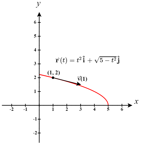
Figure \(\PageIndex{1}\): This graph depicts the velocity vector at time \(t=1\) for a particle moving in a parabolic path. - To find the parametric equations of the tangent line, we need the point at which it is tangent to the curve and a direction vector for the line. The point is just what we found above, \((1,2)\). And it turns out that we can use the velocity vector as a direction vector for the tangent line. This is always true, unless the velocity is the zero vector at this point.
So as we found above, \(\vecs v(1) = 2\hat{\mathbf i}−\frac{1}{2}\hat{\mathbf j}.\) This is the direction vector for this tangent line so we can write the parametric equations of the tangent line as: \[ \begin{align*} x &= 1+2t \\ y &= 2 - \frac{1}{2}t \\z &= 0 \end{align*}\]
A corresponding vector parameterization of this tangent line would be: \[ \vecs L(t) = \left(1+2t\right) \mathbf{\hat i} + \left(2 - \frac{1}{2}t\right) \mathbf{\hat j}. \]
Exercise \(\PageIndex{1}\)
A particle moves in a path defined by the vector-valued function \(\vecs r(t)=(t^2−3t)\,\hat{\mathbf i}+(2t−4)\,\hat{\mathbf j}+(t+2)\,\hat{\mathbf k}\), where \(t\) measures time in seconds and where distance is measured in feet. Find the velocity, acceleration, and speed as functions of time.
- Hint
-
Use Equations \ref{Eq1}, \ref{Eq2}, and \ref{Eq3}.
- Answer
-
\[\begin{align*}\vecs v(t)=\vecs{r}^{\,\prime}(t)&=(2t-3)\,\hat{\mathbf i}+2\,\hat{\mathbf j}+\,\hat{\mathbf k}\\ \vecs a(t)&=\vecs v^{\,\prime}(t) =2\,\hat{\mathbf i} \end{align*}\]
\[ ||\vecs{r}^{\,\prime}(t)||=\sqrt{(2t-3)^2+2^2+1^2} =\sqrt{4t^2-12t+14}\]
The units for velocity and speed are feet per second, and the units for acceleration are feet per second squared.
To gain a better understanding of the velocity and acceleration vectors, imagine you are driving along a curvy road. If you do not turn the steering wheel, you would continue in a straight line and run off the road. The speed at which you are traveling when you run off the road, coupled with the direction, gives a vector representing your velocity, as illustrated in Figure \(\PageIndex{2}\).
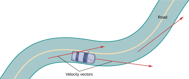
Figure \(\PageIndex{2}\): At each point along a road traveled by a car, the velocity vector of the car is tangent to the path traveled by the car.
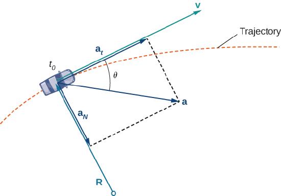
However, the fact that you must turn the steering wheel to stay on the road indicates that your velocity is always changing (even if your speed is not) because your direction is constantly changing to keep you on the road. As you turn to the right, your acceleration vector also points to the right. As you turn to the left, your acceleration vector points to the left. This indicates that your velocity and acceleration vectors are constantly changing, regardless of whether your actual speed varies (Figure \(\PageIndex{3}\)).
Projectile Motion
Now let’s look at an application of vector functions. In particular, let’s consider the effect of gravity on the motion of an object as it travels through the air, and how it determines the resulting trajectory of that object. In the following, we ignore the effect of air resistance. This situation, with an object moving with an initial velocity but with no forces acting on it other than gravity, is known as projectile motion. It describes the motion of objects from golf balls to baseballs, and from arrows to cannonballs.
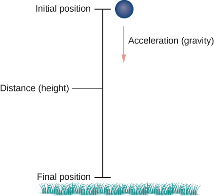
First we need to choose a coordinate system. If we are standing at the origin of this coordinate system, then we choose the positive \(y\)-axis to be up, the negative \(y\)-axis to be down, and the positive \(x\)-axis to be forward (i.e., away from the thrower of the object). The effect of gravity is in a downward direction, so Newton’s second law tells us that the force on the object resulting from gravity is equal to the mass of the object times the acceleration resulting from gravity, or \(\vecs F_g=m\vecs a\), where \(\vecs F_g\) represents the force from gravity and \(\vecs a = -g\,\hat{\mathbf j}\) represents the acceleration resulting from gravity at Earth’s surface. The value of \(g\) in the English system of measurement is approximately 32 ft/sec2 and it is approximately 9.8 m/sec2 in the metric system. This is the only force acting on the object. Since gravity acts in a downward direction, we can write the force resulting from gravity in the form \(\vecs F_g=−mg\,\hat{\mathbf j}\), as shown in Figure \(\PageIndex{4}\).
Newton’s second law also tells us that \(F=m\vecs{a}\), where \(\vecs a\) represents the acceleration vector of the object. This force must be equal to the force of gravity at all times, so we therefore know that
\[\begin{align*} \vecs F&=\vecs F_g \\ m\vecs{a} &= -mg \,\hat{\mathbf j} \\ \vecs{a} &= -g\,\hat{\mathbf j}. \end{align*}\]
Now we use the fact that the acceleration vector is the first derivative of the velocity vector. Therefore, we can rewrite the last equation in the form
\[\vecs v^{\,\prime}(t) = -g\,\hat{\mathbf j} \]
By taking the antiderivative of each side of this equation we obtain
\[ \vecs v(t) = \int -g \,\hat{\mathbf j}\; dt = -gt\,\hat{\mathbf j} + \vecs C_1 \]
for some constant vector \(\vecs C_1\). To determine the value of this vector, we can use the velocity of the object at a fixed time, say at time \(t=0\). We call this velocity the initial velocity: \(\vecs v(0)=\vecs v_0\). Therefore, \(\vecs v(0)=−g(0)\,\hat{\mathbf j}+\vecs C_1=\vecs v_0\) and \(\vecs C_1= \vecs v_0\). This gives the velocity vector as \(\vecs v(t)=−gt\,\hat{\mathbf j}+\vecs v_0\).
Next we use the fact that velocity \(\vecs{v}(t)\) is the derivative of position \(\vecs{s}(t)\). This gives the equation
\[\vecs s^{\,\prime}(t)=-gt\,\hat{\mathbf j}+\vecs{v}_0. \]
Taking the antiderivative of both sides of this equation leads to
\[\begin{align*} \vecs s(t) &= \int -gt\,\hat{\mathbf j} + \vecs{v}_0 \;dt \\ &= -\dfrac{1}{2}gt^2 \,\hat{\mathbf j} + \vecs{v}_0 t + \vecs{C}_2 \end{align*}\]
with another unknown constant vector \(\vecs{C}_2\). To determine the value of \(\vecs{C}_2\), we can use the position of the object at a given time, say at time \(t=0\). We call this position the initial position: \(\vecs{s}(0)=\vecs{s}_0\). Therefore, \(\vecs{s}(0)=−(1/2)g(0)^2\,\hat{\mathbf j}+\vecs{v}_0(0)+\vecs{C}_2=\vecs{s}_0\). This gives the position of the object at any time as
\[ \vecs{s}(t)=−\dfrac{1}{2}gt^2 \,\hat{\mathbf j}+\vecs{v}_0 t+\vecs{s}_0. \]
Let’s take a closer look at the initial velocity and initial position. In particular, suppose the object is thrown upward from the origin at an angle \(\theta\) to the horizontal, with initial speed \(\vecs{v}_0\). How can we modify the previous result to reflect this scenario? First, we can assume it is thrown from the origin. If not, then we can move the origin to the point from where it is thrown. Therefore, \(\vecs{s}_0=\vecs{0}\), as shown in Figure \(\PageIndex{5}\).
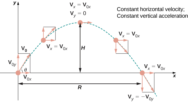
We can rewrite the initial velocity vector in the form \(\vecs{v}_0= v_0 \cos \theta \,\hat{\mathbf i} + v_0 \sin \theta \,\hat{\mathbf j}\). Then the equation for the position function \(\vecs{s}(t)\) becomes
\[\begin{align*} \vecs{s}(t)&=-\dfrac{1}{2} gt^2\,\hat{\mathbf j} + v_0 t \cos\theta \,\hat{\mathbf i} + v_0 t \sin\theta \,\hat{\mathbf j} \\ &= v_0 t \cos\theta\,\hat{\mathbf i} + v_0 t \sin\theta \,\hat{\mathbf j} - \dfrac{1}{2} gt^2\,\hat{\mathbf j} \\ &= v_0 t \cos\theta \,\hat{\mathbf i} + \left(v_0 t \sin\theta - \dfrac{1}{2} gt^2\right)\,\hat{\mathbf j}. \end{align*}\]
The coefficient of \(\hat{\mathbf i}\) represents the horizontal component of \(\vecs{s}(t)\) and is the horizontal distance of the object from the origin at time \(t\). The maximum value of the horizontal distance (measured at the same initial and final altitude) is called the range \(R\). The coefficient of \(\hat{\mathbf j}\) represents the vertical component of \(\vecs{s}(t)\) and is the altitude of the object at time \(t\). The maximum value of the vertical distance is the height \(H\).
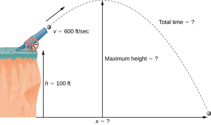
Example \(\PageIndex{2}\): Motion of a Cannonball
During an Independence Day celebration, a cannonball is fired from a cannon on a cliff toward the water. The cannon is aimed at an angle of 30° above horizontal and the initial speed of the cannonball is 600 ft/sec. The cliff is 100 ft above the water (Figure \(\PageIndex{6}\)).
- Find the maximum height of the cannonball.
- How long will it take for the cannonball to splash into the sea?
- How far out to sea will the cannonball hit the water?
Solution
We use the equation
\[\vecs{s}(t) = v_0 t \cos\theta \,\hat{\mathbf i} + \left(v_0 t \sin\theta - \dfrac{1}{2}gt^2 \right)\,\hat{\mathbf j} \]
with \(\theta=30^\circ \), \(g=32 \dfrac{\text{ft}}{\text{sec}^2}\), and \(v_0=600 \dfrac{\text{ft}}{\text{sec}}\). Then the position equation becomes
\[\begin{align*} \vecs{s}(t) &= 600 t ( \cos 30^\circ)\,\hat{\mathbf i} + \left(600t \sin30^\circ - \dfrac{1}{2}(32)t^2 \right)\,\hat{\mathbf j} \\ &= 300t\sqrt{3} \,\hat{\mathbf i} + \left( 300t - 16t^2 \right)\,\hat{\mathbf j} \end{align*}\]
- The cannonball reaches its maximum height when the vertical component of its velocity is zero, because the cannonball is neither rising nor falling at that point. The velocity vector is
\[\begin{align*} \vecs{v}(t)&=\vecs s^{\,\prime}(t)\\ &= 300 \sqrt{3} \,\hat{\mathbf i} + (300-32t)\,\hat{\mathbf j} \end{align*} \]
Therefore, the vertical component of velocity is given by the expression \(300−32t\). Setting this expression equal to zero and solving for \(t\) gives \(t=9.375\) sec. The height of the cannonball at this time is given by the vertical component of the position vector, evaluated at \(t=9.375\).\[\begin{align*} \vecs{s}(9.375)=300(9.375)\sqrt{3}\,\hat{\mathbf i}+(300(9.375)−16(9.375)^2)\,\hat{\mathbf j}=4871.39 \,\hat{\mathbf i}+1406.25\,\hat{\mathbf j} \end{align*}\]
Therefore, the maximum height of the cannonball is 1406.39 ft above the cannon, or 1506.39 ft above sea level. - When the cannonball lands in the water, it is 100 ft below the cannon. Therefore, the vertical component of the position vector is equal to \(−100.\) Setting the vertical component of \(\vecs s(t)\) equal to \(−100\) and solving, we obtain
\[\begin{align*} 300t-16t^2 &= -100 \\ 16t^2-300t-100&=0 \\4t^2-75-25&=0 \\ t&= \dfrac{75\pm \sqrt{(-75)^2}-4(4)(-25) }{2(4)} \\ &= \dfrac{75 \pm \sqrt{6025}}{8} \\ &= \dfrac{75 \pm 5\sqrt{241}}{8} \end{align*}\]
The positive value of \(t\) that solves this equation is approximately 19.08. Therefore, the cannonball hits the water after approximately 19.08 sec. - To find the distance out to sea, we simply substitute the answer from part (b) into \(\vecs{s}(t)\):
\[\begin{align*} \vecs s(19.08)&=300(19.08)\sqrt{3} \,\hat{\mathbf i}+\left(300(19.08)−16(19.08)^2\right)\,\hat{\mathbf j}\\ &=9914.26\,\hat{\mathbf i}−100.7424\,\hat{\mathbf j} \end{align*}\]
Therefore, the ball hits the water about 9914.26 ft away from the base of the cliff. Notice that the vertical component of the position vector is very close to −100, which tells us that the ball just hit the water. Note that 9914.26 feet is not the true range of the cannon since the cannonball lands in the ocean at a location below the cannon. The range of the cannon would be determined by finding how far out the cannonball is when its height is 100 ft above the water (the same as the altitude of the cannon).
Exercise \(\PageIndex{2}\)
An archer fires an arrow at an angle of 40° above the horizontal with an initial speed of 98 m/sec. The height of the archer is 171.5 cm. Find the horizontal distance the arrow travels before it hits the ground.
- Hint
-
The equation for the position vector needs to account for the height of the archer in meters.
- Answer
-
967.15 m
One final question remains: In general, what is the maximum distance a projectile can travel, given its initial speed? To determine this distance, we assume the projectile is fired from ground level and we wish it to return to ground level. In other words, we want to determine an equation for the range. In this case, the equation of projectile motion is
\[\vecs{s}=v_0 t \cos\theta \,\hat{\mathbf i} + \left(v_0t\sin\theta - \dfrac{1}{2}gt^2 \right)\,\hat{\mathbf j}.\]
Setting the second component equal to zero and solving for \(t\) yields
\[\begin{align*} v_0 t \sin\theta - \dfrac{1}{2}gt^2& =0\\ t\left(v_0 \sin\theta - \dfrac{1}{2}gt\right) &=0 \end{align*}\]
Therefore, either \(t=0\) or \(t=\dfrac{2v_0\sin\theta}{g}\). We are interested in the second value of \(t\), so we substitute this into \(\vecs{s}(t)\), which gives
\[\begin{align*} \vecs{s}\left(\dfrac{2v_0\sin\theta}{g} \right) &= v_0 \left(\dfrac{2v_0\sin\theta}{g} \right) \cos\theta \,\hat{\mathbf i} + \left( v_0\left(\dfrac{2v_0\sin\theta}{g} \right)\sin\theta - \dfrac{1}{2}g\left(\dfrac{2v_0\sin\theta}{g} \right)^2 \right)\,\hat{\mathbf j} \\ &= \left(\dfrac{2v_0^2\sin\theta\cos\theta}{g} \right)\,\hat{\mathbf i} \\ &= \dfrac{v_0^2 \sin2\theta}{g}\,\hat{\mathbf i}. \end{align*}\]
Thus, the expression for the range of a projectile fired at an angle \(\theta\) is
\[R=\dfrac{v_0^2 \sin2\theta}{g}\,\hat{\mathbf i} . \]
The only variable in this expression is \( \theta\). To maximize the distance traveled, take the derivative of the coefficient of \(\hat{\mathbf i}\) with respect to \(\theta\) and set it equal to zero:
\[\begin{align*} \dfrac{d}{d\theta} \left( \dfrac{v_0^2 \sin2\theta}{g} \right)&=0\\ \dfrac{2v_0^2\cos2\theta}{g}&=0\\ \theta=45^\circ \end{align*}\]
This value of \(\theta)\) is the smallest positive value that makes the derivative equal to zero. Therefore, in the absence of air resistance, the best angle to fire a projectile (to maximize the range) is at a 45° angle. The distance it travels is given by
\[\vecs{s}\left(\dfrac{2v_0 \sin 45^\circ}{g} \right)= \dfrac{v_0^2 \sin 90^\circ}{g} \,\hat{\mathbf i} = \dfrac{v_0^2}{g}\,\hat{\mathbf i} \]
Therefore, the range for an angle of 45° is \(\dfrac{v_0^2}{g}\) units.
Key Concepts
- If \(\vecs{r}(t)\) represents the position of an object at time \(t,\) then \(\vecs{r}^{\,\prime}(t)\) represents the velocity and \(\vecs{r}′^{\,\prime}(t)\) represents the acceleration of the object at time \(t.\) The magnitude of the velocity vector is speed.
- Projectile motion can be represented by the vector-valued function \[\vecs{r}(t) = v_0 t \cos\theta \,\hat{\mathbf i} + \left(v_0 t \sin\theta - \dfrac{1}{2}gt^2 \right)\,\hat{\mathbf j}, \] where the initial velocity is given by \(\vecs{v}_0= v_0 \cos \theta \,\hat{\mathbf i} + v_0 \sin \theta \,\hat{\mathbf j}\).
Key Equations
- Velocity \[\vecs{v}(t)=\vecs{r}^{\,\prime}(t) \nonumber\]
- Acceleration \[\vecs{a}(t)=\vecs{v}^{\,\prime}(t)=\vecs{r}′^{\,\prime}(t) \nonumber\]
- Speed \[v(t)=||\vecs{v}(t)||=||\vecs{r}^{\,\prime}(t)||=\dfrac{ds}{dt} \nonumber\]
- Projectile Motion \[\vecs{r}(t) = v_0 t \cos\theta \,\hat{\mathbf i} + \left(v_0 t \sin\theta - \dfrac{1}{2}gt^2 \right)\,\hat{\mathbf j} \]
Glossary
- acceleration vector
- the second derivative of the position vector
- projectile motion
- motion of an object with an initial velocity but no force acting on it other than gravity
- velocity vector
- the derivative of the position vector
Contributors
Gilbert Strang (MIT) and Edwin “Jed” Herman (Harvey Mudd) with many contributing authors. This content by OpenStax is licensed with a CC-BY-SA-NC 4.0 license. Download for free at http://cnx.org.
- Edited by Paul Seeburger
Paul Seeburger added finding point \((1, 2)\) when \(t=1\) and added part 3 (finding the equations of the tangent line) in Example \(\PageIndex{1}\).
He also created Figure \(\PageIndex{1}\).