Vector-Valued Functions and Space Curves

Our study of vector-valued functions combines ideas from our earlier examination of single-variable calculus with our description of vectors in three dimensions from the preceding chapter. In this section, we extend concepts from earlier chapters and also examine new ideas concerning curves in three-dimensional space. These definitions and theorems support the presentation of material in the rest of this chapter and also in the remaining chapters of the text.

Definition of a Vector-Valued Function

Our first step in studying the calculus of vector-valued functions is to define what exactly a vector-valued function is. We can then look at graphs of vector-valued functions and see how they define curves in both two and three dimensions.

Definition: Vector-valued Functions

A vector-valued function is a function of the form

$$\vecs r(t)=f(t)\,\hat{\mathbf{i}}+g(t)\,\hat{\mathbf{j}} \quad \text{or} \quad \vecs r(t)=f(t)\,\hat{\mathbf{i}}+g(t)\,\hat{\mathbf{j}}+h(t)\,\hat{\mathbf{k}},$$

where the component functions $f$, $g$, and $h$, are real-valued functions of the parameter $t$.

Vector-valued functions can also be written in the form

$$\vecs r(t)=⟨f(t),\,g(t)⟩ \; \; \text{or} \; \; \vecs r(t)=⟨f(t),\,g(t),\,h(t)⟩.$$

In both cases, the first form of the function defines a two-dimensional vector-valued function in the plane; the second form describes a three-dimensional vector-valued function in space.

We often use $t$ as a parameter because $t$ can represent time.

The parameter $t$ may lie between two real numbers: $a≤t≤b$, or its value may range over the entire set of real numbers.

Each of the component functions that make up a vector-valued function may have domain restrictions that enforce restrictions on the value of $t$.

The domain of a vector-valued function $\vecs r$ is the intersection of the domains of its component functions, i.e., it is the set of all values of $t$ for which the vector-valued function is defined.

Example $\PageIndex{1}$: Finding the domain of a vector-valued function

State the domain of the vector-valued function $\vecs r(t)=\sqrt{2-t} \,\hat{\mathbf{i}}+\ln(t+3)\,\hat{\mathbf{j}} + e^t \, \hat{\mathbf{k}}$.

Solution

We first consider the natural domain of each component function. Note that we list the domains in both set-builder notation and interval notation.

Function: Domain:
$\begin{array}{ll} \sqrt{2-t} & & \big\{\,t\,|\, t \le 2\big\} \quad \text{or} \quad (-\infty, 2\big] \\ \ln(t+3) & & \big\{\,t\,|\, t \gt -3\big\} \quad \text{or} \quad (-3, \infty ) \\ e^t & & (-\infty, \infty) \end{array}$

The domain of $\vecs r$ is the intersection of these domains, so it must contain all values of $t$ that work in all three, but no value of $t$ that does not work in any one of these functions.

Hence, the domain of $\vecs r$ is: $\text{D}_{\vecs r}: \big\{\,t\,|\, -3 \lt t \le 2\big\}$ or $(-3, 2\big]$.

Note that only one form of the domain of $\vecs r$ need be given. The first, $\big\{\,t\,|\, -3 \lt t \le 2\big\}$, is in set-builder notation, while the second, $(-3, 2\big]$, is in interval notation.

Example $\PageIndex{2}$: Evaluating Vector-Valued Functions and Determining Domains

For each of the following vector-valued functions, evaluate $\vecs r(0)$, $\vecs r(\frac{\pi}{2})$, and $\vecs r(\frac{2\pi}{3})$. Do any of these functions have domain restrictions?

1. $\vecs r(t)=4\cos t\,\hat{\mathbf{i}}+3\sin t\,\hat{\mathbf{j}}$
2. $\vecs r(t)=3\tan t\,\hat{\mathbf{i}}+4 \sec t\,\hat{\mathbf{j}}+5t\,\hat{\mathbf{k}}$

Solution

1. To calculate each of the function values, substitute the appropriate value of $t$ into the function:

   $$\begin{align*}\vecs r(0) \; & = 4\cos(0) \hat{\mathbf{i}}+3\sin(0) \hat{\mathbf{j}} \\[4pt] & =4\hat{\mathbf{i}}+0 \hat{\mathbf{j}}=4\hat{\mathbf{i}} \\[4pt] \vecs r\left(\frac{\pi}{2}\right) \; & = 4\cos\left(\frac{π}{2}\right)\hat{\mathbf{i}}+3\sin\left(\frac{π}{2}\right) \hat{\mathbf{j}} \\[4pt] & = 0\hat{\mathbf{i}}+3 \hat{\mathbf{j}}=3 \hat{\mathbf{j}} \\[4pt] \vecs r\left(\frac{2\pi}{3}\right) \; & =4\cos\left(\frac{2π}{3}\right)\hat{\mathbf{i}}+3\sin\left(\frac{2π}{3}\right) \hat{\mathbf{j}} \\[4pt] & =4\left(−\tfrac{1}{2}\right)\hat{\mathbf{i}}+3\left(\tfrac{\sqrt{3}}{2}\right) \hat{\mathbf{j}}=−2 \hat{\mathbf{i}}+\tfrac{3 \sqrt{3}}{2} \hat{\mathbf{j}}\end{align*}$$

   To determine whether this function has any domain restrictions, consider the component functions separately. The first component function is $f(t)=4 \cos t$ and the second component function is $g(t)=3\sin t$. Neither of these functions has a domain restriction, so the domain of $\vecs r(t)=4\cos t\,\hat{\mathbf{i}}+3 \sin t \,\hat{\mathbf{j}}$ is all real numbers.
2. To calculate each of the function values, substitute the appropriate value of t into the function: $$\begin{align*}\vecs r(0) \; & = 3\tan(0)\hat{\mathbf{i}}+4\sec(0) \hat{\mathbf{j}}+5(0) \hat{\mathbf{k}} \\[4pt] & = 0\hat{\mathbf{i}}+4j+0 \hat{\mathbf{k}}=4 \hat{\mathbf{j}} \\[4pt] \vecs r\left(\frac{\pi}{2}\right) \; & = 3\tan\left(\frac{\pi}{2}\right)\hat{\mathbf{i}}+4\sec\left(\frac{\pi}{2}\right) \hat{\mathbf{j}}+5\left(\frac{\pi}{2}\right) \hat{\mathbf{k}},\,\text{which does not exist} \\[4pt] \vecs r\left(\frac{2\pi}{3}\right) \; & =3\tan\left(\frac{2 \pi}{3}\right)\hat{\mathbf{i}}+4\sec\left(\frac{2\pi}{3}\right) \hat{\mathbf{j}}+5\left(\frac{2\pi}{ 3}\right) \hat{\mathbf{k}} \\[4pt] & =3(−\sqrt{3})\hat{\mathbf{i}}+4(−2)\hat{\mathbf{j}}+\frac{10π}{3} \hat{\mathbf{k}} \\[4pt] & =(-3\sqrt{3})\hat{\mathbf{i}}−8\hat{\mathbf{j}}+\frac{10π}{3} \hat{\mathbf{k}}\end{align*}$$ To determine whether this function has any domain restrictions, consider the component functions separately. The first component function is $f(t)=3\tan t$, the second component function is $g(t)=4\sec t$, and the third component function is $h(t)=5t$. The first two functions are not defined for odd multiples of $\frac{\pi}{2}$, so the function is not defined for odd multiples of $\frac{\pi}{2}$. Therefore, $$\text{D}_{\vecs r}=\Big\{t\,|\,t≠ \frac{(2n+1)\pi}{2}\Big\},\nonumber$$ where $n$ is any integer.

Exercise $\PageIndex{1}$

For the vector-valued function $\vecs r(t)=(t^2−3t) \,\hat{\mathbf{i}}+(4t+1) \,\hat{\mathbf{j}}$, evaluate $\vecs r(0),\, \vecs r(1)$, and $\vecs r(−4)$. Does this function have any domain restrictions?

Hint

Substitute the appropriate values of $t$ into the function.

Answer

$\vecs r(0) = \hat{\mathbf{j}},\, \vecs r(1)=−2 \hat{\mathbf{i}}+5 \hat{\mathbf{j}},\, \vecs r(−4)=28 \hat{\mathbf{i}}−15 \hat{\mathbf{j}}$

The domain of $\vecs r(t)=(t^2−3t)\hat{\mathbf{i}}+(4t+1)\hat{\mathbf{j}}$ is all real numbers.

Example $\PageIndex{1}$ illustrates an important concept. The domain of a vector-valued function consists of real numbers. The domain can be all real numbers or a subset of the real numbers. The range of a vector-valued function consists of vectors. Each real number in the domain of a vector-valued function is mapped to either a two- or a three-dimensional vector.

Graphing Vector-Valued Functions

Recall that a plane vector consists of two quantities: direction and magnitude. Given any point in the plane (the initial point), if we move in a specific direction for a specific distance, we arrive at a second point. This represents the terminal point of the vector. We calculate the components of the vector by subtracting the coordinates of the initial point from the coordinates of the terminal point.

A vector is considered to be in standard position if the initial point is located at the origin. When graphing a vector-valued function, we typically graph the vectors in the domain of the function in standard position, because doing so guarantees the uniqueness of the graph. This convention applies to the graphs of three-dimensional vector-valued functions as well. The graph of a vector-valued function of the form

$$\vecs r(t)=f(t)\, \hat{\mathbf{i}}+g(t)\,\hat{\mathbf{j}} \nonumber$$

consists of the set of all points $(f(t),\,g(t))$, and the path it traces is called a plane curve. The graph of a vector-valued function of the form

$$\vecs r(t)=f(t) \,\hat{\mathbf{i}}+g(t) \,\hat{\mathbf{j}}+h(t) \,\hat{\mathbf{k}} \nonumber$$

consists of the set of all points $(f(t),\,g(t),\,h(t))$, and the path it traces is called a space curve. Any representation of a plane curve or space curve using a vector-valued function is called a vector parameterization of the curve.

Each plane curve and space curve has an orientation, indicated by arrows drawn in on the curve, that shows the direction of motion along the curve as the value of the parameter $t$ increases.

Example $\PageIndex{3}$: Graphing a Vector-Valued Function

Create a graph of each of the following vector-valued functions:

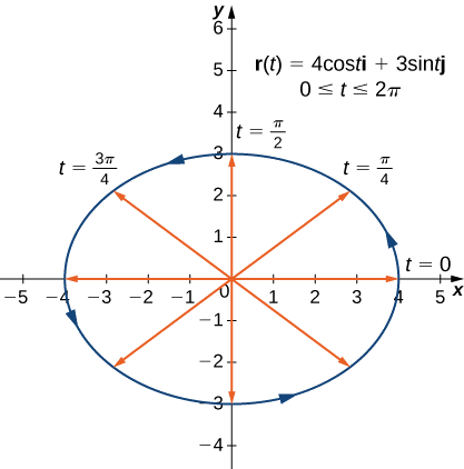
1. The plane curve represented by $\vecs r(t)=4 \cos t \,\hat{\mathbf{i}}+3 \sin t \,\hat{\mathbf{j}}$, $0≤t≤2\pi$
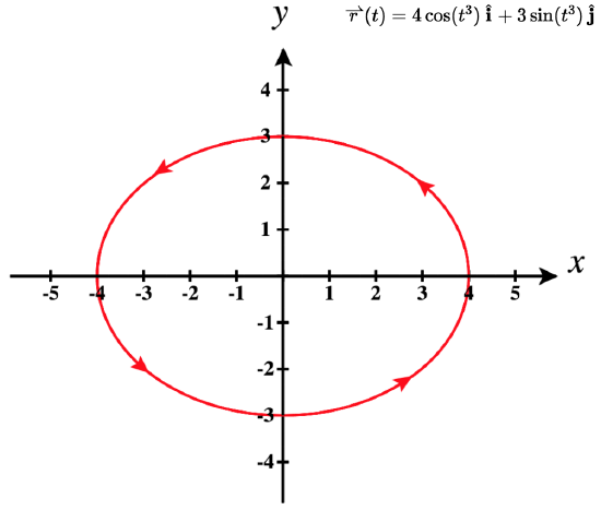
2. The plane curve represented by $\vecs r(t)=4 \cos(t^3) \,\hat{\mathbf{i}}+3 \sin(t^3) \,\hat{\mathbf{j}}$, $0≤t≤\sqrt[3]{2\pi}$
3. The space curve represented by $\vecs r(t)=4 \cos t \,\hat{\mathbf{i}}+4 \sin t \,\hat{\mathbf{j}}+t \,\hat{\mathbf{k}}$, $0≤t≤4\pi$

Solution

a. As with any graph, we start with a table of values. We then graph each of the vectors in the second column of the table in standard position and connect the terminal points of each vector to form a curve (Figure $\PageIndex{1}$). This curve turns out to be an ellipse centered at the origin.

Table $\PageIndex{1}$: Table of Values for $\vecs r(t)=4 \cos t \,\hat{\mathbf{i}}+3 \sin t \,\hat{\mathbf{j}}$, $0≤t≤2\pi$

$t$	$\vecs r(t)$	$t$	$\vecs r(t)$
$0$	$4\hat{\mathbf{i}}$	$\pi$	$-4\hat{\mathbf{i}}$
$\dfrac{\pi}{4}$	$2 \sqrt{2} \hat{\mathbf{i}} + \frac{3 \sqrt{2}}{2}\hat{\mathbf{j}}$	$\dfrac{5\pi}{4}$	$-2 \sqrt{2} \hat{\mathbf{i}} - \frac{3 \sqrt{2}}{2}\hat{\mathbf{j}}$
$\dfrac{\pi}{2}$	$\mathrm{3\hat{\mathbf{j}}}$	$\dfrac{3\pi}{2}$	$\mathrm{-3\hat{\mathbf{j}}}$
$\dfrac{3\pi}{4}$	$-2 \sqrt{2} \hat{\mathbf{i}} + \frac{3 \sqrt{2}}{2}\hat{\mathbf{j}}$	$\dfrac{7\pi}{4}$	$2 \sqrt{2} \hat{\mathbf{i}} - \frac{3 \sqrt{2}}{2}\hat{\mathbf{j}}$
$2\pi$	$4\hat{\mathbf{i}}$

Figure $\PageIndex{1}$: The graph of the first vector-valued function is an ellipse.

b. The table of values for $\vecs r(t)=4 \cos(t^3) \,\hat{\mathbf{i}}+3 \sin(t^3) \,\hat{\mathbf{j}}$, $0≤t≤\sqrt[3]{2\pi}$ is as follows:

Table of Values for $\vecs r(t)=4 \cos(t^3) \,\hat{\mathbf{i}}+3 \sin(t^3) \,\hat{\mathbf{j}}$, $0≤t≤\sqrt[3]{2\pi}$

$t$	$\vecs r(t)$	$t$	$\vecs r(t)$
$0$	$\mathrm{4\hat{\mathbf{i}}}$	$\displaystyle\sqrt[3]{\pi}$	$\mathrm{-4\hat{\mathbf{i}}}$
$\displaystyle \sqrt[3]{\dfrac{\pi}{4}}$	$\mathrm{ 2 \sqrt{2} \hat{\mathbf{i}} + \frac{3 \sqrt{2}}{2}\hat{\mathbf{j}}}$	$\displaystyle \sqrt[3]{\dfrac{5\pi}{4}}$	$\mathrm{ -2 \sqrt{2} \hat{\mathbf{i}} - \frac{3 \sqrt{2}}{2}\hat{\mathbf{j}}}$
$\displaystyle \sqrt[3]{\dfrac{\pi}{2}}$	$\mathrm{3\hat{\mathbf{j}}}$	$\displaystyle \sqrt[3]{\dfrac{3\pi}{2}}$	$\mathrm{-3\hat{\mathbf{j}}}$
$\displaystyle \sqrt[3]{\dfrac{3\pi}{4}}$	$\mathrm{ -2 \sqrt{2} \hat{\mathbf{i}} + \frac{3 \sqrt{2}}{2}\hat{\mathbf{j}}}$	$\displaystyle \sqrt[3]{\dfrac{7\pi}{4}}$	$\mathrm{ 2 \sqrt{2} \hat{\mathbf{i}} - \frac{3 \sqrt{2}}{2}\hat{\mathbf{j}}}$
$\displaystyle\sqrt[3]{2\pi}$	$\mathrm{4\hat{\mathbf{i}}}$

The graph of this curve is also an ellipse centered at the origin.

Figure $\PageIndex{2}$: The graph of the second vector-valued function is also an ellipse.

c. We go through the same procedure for a three-dimensional vector function.

Table of Values for $\mathrm{r(t)= 4 \cos t \hat{\mathbf{i}}+4 \sin t \hat{\mathbf{j}}+t \hat{\mathbf{k}}}$, $\mathrm{0≤t≤4\pi}$

$t$	$\vecs r(t)$	$t$	$\vecs r(t)$
$\mathrm{0}$	$\mathrm{4\hat{\mathbf{i}}}$	$\mathrm{\pi}$	$\mathrm{-4\hat{\mathbf{i}}}+ \pi \hat{\mathbf{k}}$
$\dfrac{\pi}{4}$	$\mathrm{2 \sqrt{2} \hat{\mathbf{i}} + 2\sqrt{2} \hat{\mathbf{j}} + \frac{\pi}{4} \hat{\mathbf{k}}}$	$\dfrac{5\pi}{4}$	$\mathrm{ -2 \sqrt{2} \hat{\mathbf{i}} - 2\sqrt{2} \hat{\mathbf{j}} + \frac{5\pi}{4} \hat{\mathbf{k}}}$
$\dfrac{\pi}{2}$	$\mathrm{4\hat{\mathbf{j}} +\frac{\pi}{2} \hat{\mathbf{k}}}$	$\dfrac{3\pi}{2}$	$\mathrm{-4\hat{\mathbf{j}} +\frac{3\pi}{2} \hat{\mathbf{k}}}$
$\dfrac{3\pi}{4}$	$\mathrm{ -2 \sqrt{2} \hat{\mathbf{i}} + 2\sqrt{2} \hat{\mathbf{j}} + \frac{3\pi}{4} \hat{\mathbf{k}}}$	$\dfrac{7\pi}{4}$	$\mathrm{ 2 \sqrt{2} \hat{\mathbf{i}} - 2\sqrt{2} \hat{\mathbf{j}} + \frac{7\pi}{4} \hat{\mathbf{k}}}$
$\mathrm{2\pi}$	$\mathrm{4\hat{\mathbf{j}} + 2\pi \hat{\mathbf{k}}}$

The values then repeat themselves, except for the fact that the coefficient of $\hat{\mathbf{k}}$ is always increasing ( $\PageIndex{3}$). This curve is called a helix. Notice that if the $\hat{\mathbf{k}}$ component is eliminated, then the function becomes $\vecs r(t)=4\cos t \hat{\mathbf{i}}+ 4\sin t \hat{\mathbf{j}}$, which is a circle of radius 4 centered at the origin.

Figure $\PageIndex{3}$: The graph of the third vector-valued function is a helix.

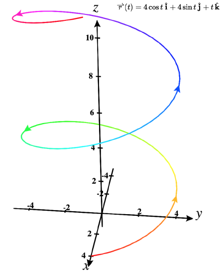
You may notice that the graphs in parts a. and b. are identical. This happens because the function describing the curve in part b. is a so-called reparameterization of the function describing the curve in part a. In fact, any curve has an infinite number of reparameterizations; for example, we can replace $t$ with $2t$ in any of the three previous curves without changing the shape of the curve. The interval over which $t$ is defined may change, but that is all. We return to this idea later in this chapter when we study arc-length parameterization. As mentioned, the name of the shape of the curve of the graph in $\PageIndex{3}$ is a helix. The curve resembles a spring, with a circular cross-section looking down along the $z$-axis. It is possible for a helix to be elliptical in cross-section as well. For example, the vector-valued function $\vecs r(t)=4 \cos t \,\hat{\mathbf{i}}+3 \sin t \,\hat{\mathbf{j}}+t \,\hat{\mathbf{k}}$ describes an elliptical helix. The projection of this helix into the $xy$-plane is an ellipse. Last, the arrows in the graph of this helix indicate the orientation of the curve as $t$ progresses from $0$ to $4π$.

Exercise $\PageIndex{2}$

Create a graph of the vector-valued function $\vecs r(t)=t \,\hat{\mathbf{i}}+ t^3 \, \hat{\mathbf{j}}$.

Hint

Start by making a table of values, then graph the points indicated by the vectors for each value of $t$.

Answer

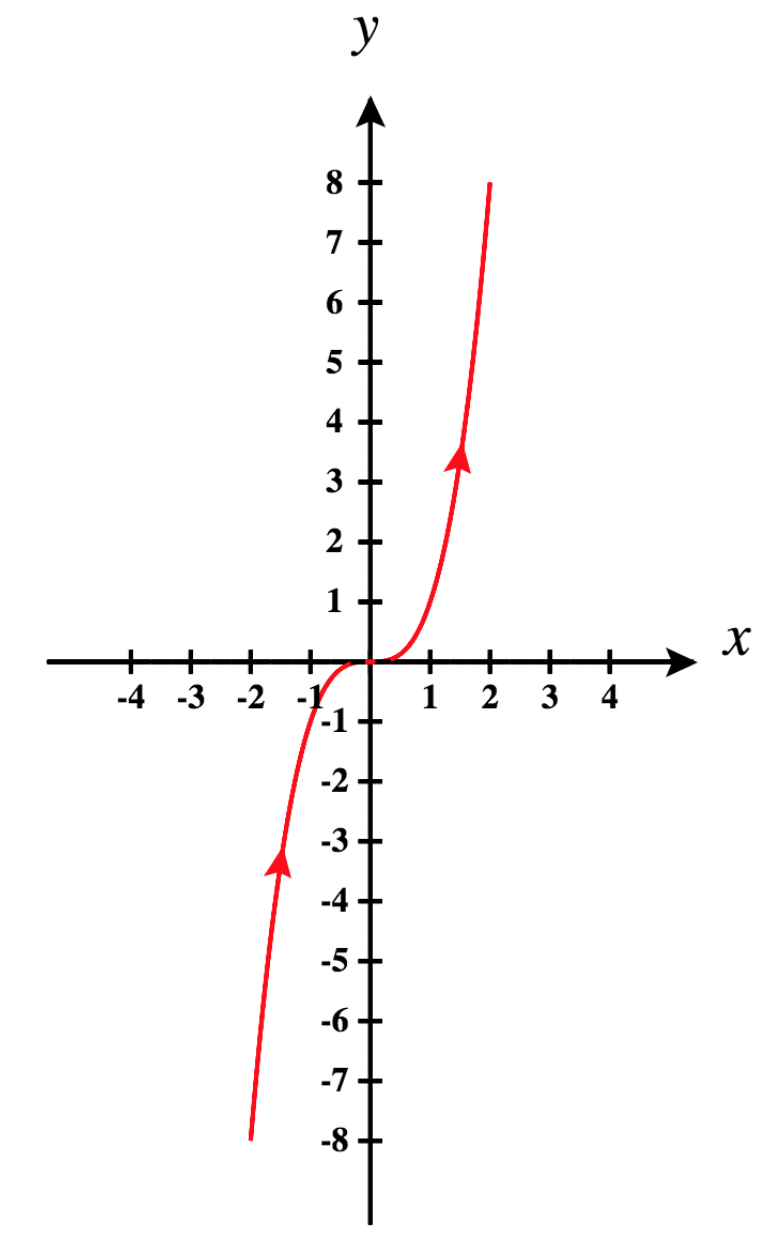
At this point, you may notice a similarity between vector-valued functions and parameterized curves. Indeed, given a vector-valued function $\vecs r(t)=f(t)\,\hat{\mathbf{i}}+g(t)\,\hat{\mathbf{j}}$ we can define $x=f(t)$ and $y=g(t)$. The graph of the parameterized function would then agree with the graph of the vector-valued function, except that the vector-valued function's graph would be traced out by vectors rather than just being a collection of points. Since we can parameterize a curve defined by a function $y=f(x)$, it is also possible to represent an arbitrary plane curve by a vector-valued function.

Finding a Vector-Valued Function to Trace out the Graph of a Function y = f(x)

As you can see in the examples above, a vector-valued function traces out a curve in the plane or in space. What if we wish to write a vector-valued function that traces out the graph of a particular curve in the $xy$-plane?

What function's graph is traced out by the vector-valued function in Exercise $\PageIndex{2}$ above: $\vecs r(t)=t \,\hat{\mathbf{i}}+ t^3 \,\hat{\mathbf{j}}$? It looks like the graph of $y = x^3$, doesn't it?

Remembering what was just said about the components of the vector-valued function corresponding to the parametic equations of a parameterized curve, we see that here we have:

$$\begin{align*} x &= t \\ y &= t^3\end{align*}\nonumber$$

Since $x = t$, we can replace $t$ in the equation $y = t^3$ with $x$, giving us the function: $y = x^3$.

So we were correct in our guess.

How could we write a vector-valued function to trace out the graph of a function, $y = f(x)$?

Well, there are two orientations to consider: left-to-right and right-to-left.

Tracing a Function from Left-To-Right:

To trace out the graph of $y = f(x)$ from left-to-right, use: $\vecs r(t) = t \,\hat{\mathbf{i}}+ f(t) \,\hat{\mathbf{j}}$

Note that what's important here is to have the $x$ component be an increasing function. Any increasing function will work. We could use $x = t^3$, for example. But then we would need to remember to replace $x$ in the function $f(x)$ with this expression $t^3$, giving us $y = f(t^3)$. This means the function $y = f(x)$ could also be parameterized from left-to-right by the vector-valued function: $\vecs r(t) = t^3 \,\hat{\mathbf{i}}+ f(t^3) \,\hat{\mathbf{j}}$

Tracing a Function from Right-To-Left:

To trace out the graph of $y = f(x)$ from right-to-left, use: $\vecs r(t) = -t \,\hat{\mathbf{i}}+ f(-t) \,\hat{\mathbf{j}}$

Again note that we could use any decreasing function of $t$ for the $x$ component and obtain a vector-valued function that traces out the graph of $y = f(x)$ from right-to-left. Using $x = -t$ is just the simplest decreasing function we can choose.

Example $\PageIndex{4}$: Finding a vector-valued function to trace the graph of $y = f(x)$

Determine a vector-valued function that will trace out the graph of $y = \cos x$ from left-to-right, and another one to trace it out from right-to-left.

Solution

Left-to-right: $\vecs r(t) = t \,\hat{\mathbf{i}}+ \cos t \,\hat{\mathbf{j}}$

Right-to-left: $\vecs r(t) = -t \,\hat{\mathbf{i}}+ \cos (-t) \,\hat{\mathbf{j}}$

Finding a Vector-Valued Function to Trace out the Graph of an Equation in x and y and Vice Versa

What if we wish to find a vector-valued function to trace out the graph of a circle, an ellipse, or a hyperbola, given its implicit equation?

Well, note that in Example $\PageIndex{3}$, the vector-valued function $\vecs r(t)=4 \cos t \,\hat{\mathbf{i}}+3 \sin t \,\hat{\mathbf{j}}$ traced out the graph of the ellipse $\frac{x^2}{16} + \frac{y^2}{9} = 1$.

In this vector-valued function we see that: $$x = 4\cos t \quad \text{and} \quad y = 3\sin t$$

What we need now is a way to convert this to an implicit equation involving $x$ and $y$. To accomplish this, remember the Pythagorean identity, $$\cos^2 t + \sin^2 t = 1$$ .

Now all we need to do is solve the above equations for $\cos t$ and $\sin t$ and we can substitute into this identity to obtain an equation in $x$ and $y$.

So: $$\cos t = \frac{x}{4} \quad \text{and} \quad \sin t = \frac{y}{3}$$

Substituting into the identity gives us: $$\left( \frac{x}{4}\right)^2 + \left( \frac{y}{3}\right)^2 = 1$$

Simplifying this implicit equation gives us the implicit equation of the ellipse in Example $\PageIndex{3}$ that we wrote above:

$$\frac{x^2}{16} + \frac{y^2}{9} = 1$$

To go the other way and find a vector-valued function that traces out an ellipse requires us to simply take these steps in the opposite direction!

Example $\PageIndex{5}$: Writing a vector-valued function for a given circle, ellipse, or Hyperbola

Write a vector-valued function that traces out each of the following implicit curves:

1. The ellipse: $\frac{x^2}{16} + \frac{y^2}{9} = 1$
2. The circle: $x^2 + y^2 = 4$
3. The hyperbola: $\frac{x^2}{25} - \frac{y^2}{16} = 1$

Solution

a. Let's just use the process shown above in reverse. First, let's rewrite the implicit equation so it shows a sum of quantities squared equals one.

$$\left( \frac{x}{4}\right)^2 + \left( \frac{y}{3}\right)^2 = 1 \nonumber$$

Now we need the identity we used above, $\cos^2 t + \sin^2 t = 1$.

Equating the parts being squared (note we actually have a choice here about which to make $\cos t$ and which to make $\sin t$), we get:

$$\frac{x}{4} = \cos t \quad \text{and} \quad \frac{y}{3} = \sin t \nonumber$$

Now we just need to solve for $x$ and $y$.

$$x = 4\cos t \quad \text{and} \quad y = 3\sin t \nonumber$$

We can now write a vector-valued function that traces out this ellipse: $\vecs r(t) = 4\cos t\,\hat{\mathbf{i}}+ 3\sin t \,\hat{\mathbf{j}}$

Note that we could also have written $\vecs r(t) = 4\sin t\,\hat{\mathbf{i}}+ 3\cos t \,\hat{\mathbf{j}}$, since we could have chosen to switch the $\sin t$ and $\cos t$ above. It will trace out the same ellipse, but with the opposite orientation.

b. Tracing out a circle is fairly straightforward, not really needing the process we showed above, although it still may be helpful at first. Remember that all the vectors on the unit circle can be represented in the form: $\vecs v = \cos \theta \, \hat{\mathbf{i}} + \sin \theta \, \hat{\mathbf{j}}$.

So the vector-valued function, $\vecs r(t) = \cos t\,\hat{\mathbf{i}}+ \sin t \,\hat{\mathbf{j}}$, will trace out the unit circle with equation, $x^2 + y^2 = 1$.

To obtain a circle of radius $2$ centered at the origin (which is the graph of $x^2 + y^2 = 4$), we just need to multiply through this vector-valued function by a scalar factor of $2$.

Thus, a vector-valued function that will trace out this circle is: $\vecs r(t) = 2\cos t\,\hat{\mathbf{i}}+ 2\sin t \,\hat{\mathbf{j}}$.

Note again that another possibility is: $\vecs r(t) = 2\sin t\,\hat{\mathbf{i}}+ 2\cos t \,\hat{\mathbf{j}}$. It will trace out the same circle, but with the opposite orientation.

To use the technique above, you start by dividing each term in the equation by the square of the radius, here 4, thus putting the circle equation in "ellipse form". The rest of the steps follow the pattern shown in part a.

c. To trace out a hyperbola of the form $\frac{x^2}{a^2} - \frac{y^2}{b^2} = 1$ or $\frac{y^2}{a^2} - \frac{x^2}{b^2} = 1$, we need to locate a trigonometric identity showing the difference of two squares equals 1. If you don't already have such an identity memorized, we can obtain one from the Pythagorean identity used above. That is,

$$\cos^2 t + \sin^2 t = 1 \nonumber$$

Dividing through each term by $\cos^2 t$

$$\frac{\cos^2 t}{\cos^2 t} + \frac{\sin^2 t}{\cos^2 t} = \frac{1}{\cos^2 t} \nonumber$$

yields,

$$1+ \tan^2 t = \sec^2 t \nonumber$$

Rewriting this equation gives us the identity we need:

$$\sec^2 t - \tan^2 t = 1 \nonumber$$

Now, the equation of this hyperbola is:

$$\frac{x^2}{25} - \frac{y^2}{16} = 1 \nonumber$$

Rewriting the left side to show the quantities that are squared:

$$\left(\frac{x}{5}\right)^2 - \left(\frac{y}{4}\right)^2 = 1 \nonumber$$

We can then equate the squared expressions corresponding terms:

$$\frac{x}{5} = \sec t \quad \text{and} \quad \frac{y}{4} = \tan t \nonumber$$

Solving for $x$ and $y$, we have:

$$x = 5\sec t \quad \text{and} \quad y = 4\tan t \nonumber$$

So a vector-valued function that will trace out the hyperbola $$\frac{x^2}{25} - \frac{y^2}{16} = 1$$ is $$\vecs r(t) = 5\sec t\,\hat{\mathbf{i}}+ 4\tan t \,\hat{\mathbf{j}}. \nonumber$$

Parameterizing a Piecewise Path

There are times when it is necessary to parameterize a path made up of pieces of different curves. This piecewise path may be open or form the boundary of a closed region as does the example shown in Figure $\PageIndex{4}$. In addition to determining a vector-valued function to trace out each piece separately, with the indicated orientation, we also need to determine a suitable range of values for the parameter $t$.

Note that there are many ways to parameterize any one piece, so there are many correct ways to parameterize a path in this way.

Example $\PageIndex{6}$: Parameterizing a piecewise path

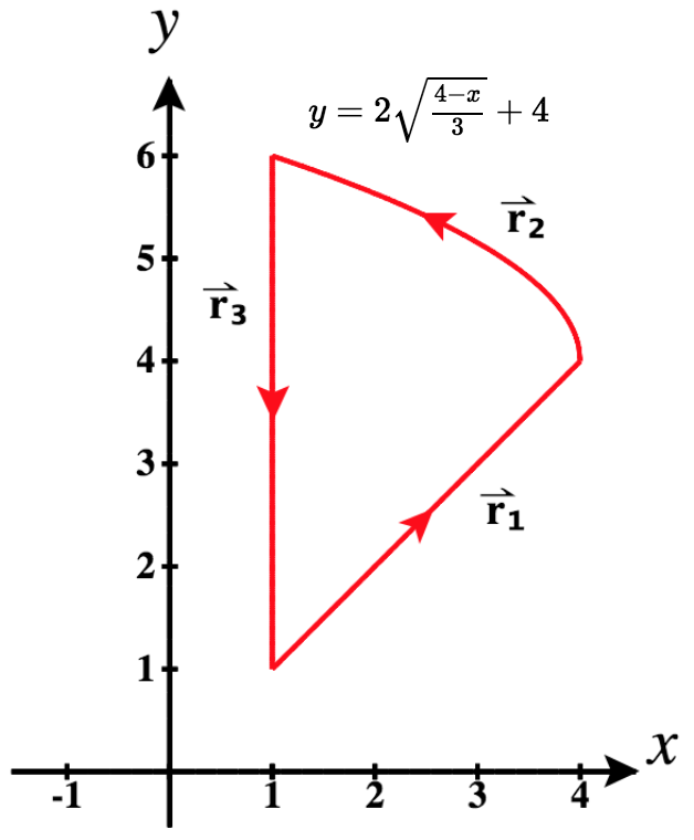Determine a piecewise parameterization of the path shown in Figure $\PageIndex{4}$, starting with $t=0$ and continuing on through each piece.

Solution

Our first task is to identify the three pieces in this piecewise path.

Note how we labeled these sequentially as $\vecs r_1$, $\vecs r_2$, and $\vecs r_3$. Now we need to identify the function for each and write the corresponding vector-valued function with the correct orientation (left-to-right or right-to-left).

Determining $\vecs r_1$: The equation of the linear function in this piece is $y = x$.

Since it is oriented from left-to-right between $t = 1$ and $t = 4$, we can write:

$$\vecs r_{1a}(t) = t\,\hat{\mathbf{i}}+ t \,\hat{\mathbf{j}} \quad\text{for}\quad 1 \le t \le 4 \nonumber$$

If we wish to begin this piece at $t = 0$, we just need to shift the value of $t$ one unit to the left. One way to do this is to write $\vecs r_{1a}$ in terms of $t_1$ instead of $t$ to make the translation easier to see.

Thus, we have $\vecs r_{1a}(t_1) = t_1\,\hat{\mathbf{i}}+ t_1 \,\hat{\mathbf{j}}$ for $1\le t_1\le 4$.

Figure $\PageIndex{4}$: A closed piecewise path

Subtracting $1$ from each part of this range of parameter values, we have: $0 \le t_1 - 1 \le 3$.

Now we let $t = t_1 - 1$. Solving for $t_1$, we obtain: $t_1 = t + 1$.

Replacing $t_1$ with the expression $t + 1$ will effectively shift the range of parameter values one unit to the left.

So, starting with $t = 0$, we have: $$\vecs r_1(t) = (t+1)\,\hat{\mathbf{i}}+ (t+1) \,\hat{\mathbf{j}} \quad\text{for}\quad 0 \le t \le 3 \nonumber$$

Double-check that this vector-valued function will trace out this segment in the correct direction before going on to $r_2$.

Determining $\vecs r_2$: This piece has a label showing the function whose graph it traces along. If it were oriented from left-to-right, we would have:

$$\text{Left-to-right:}\quad\vecs r_{2a}(t) = t\,\hat{\mathbf{i}}+ \left(2\sqrt{\frac{4-t}{3}}+4\right) \,\hat{\mathbf{j}} \quad\text{for}\quad 1 \le t \le 4 \nonumber$$

But since we need it to be oriented from right-to-left, we need to replace $t$ with $-t$ in the function and we need to divide through the range inequality by -1 to obtain the corresponding range. Thus we obtain:

$$\vecs r_{2b}(t) = -t\,\hat{\mathbf{i}}+ \left(2\sqrt{\frac{4-(-t)}{3}}+4\right) \,\hat{\mathbf{j}} \quad\text{for}\quad -4 \le t \le -1 \nonumber$$

Check that it works!

Now we wish to have this piece start at $t = 3$ just after the first one finishes. Again let's make this easier to see by writing $r_{2b}$ in terms on $t_2$.

$$\vecs r_{2b}(t_2) = -t_2\,\hat{\mathbf{i}}+ \left(2\sqrt{\frac{4-(-t_2)}{3}}+4\right) \,\hat{\mathbf{j}} \quad\text{for}\quad -4 \le t_2 \le -1 \nonumber$$

To force $r_2$ to start with $t = 3$ instead of $t = -4$, we need to add $7$ to each part of the inequality. This yields: $3 \le t_2 + 7 \le 6$.

Let $t = t_2 + 7$. Then solving for $-t_2$ (since this is what we need to replace in $r_{2b}$), we have: $-t_2 = 7-t$.

Replacing $-t_2$ with $\left(7-t\right)$ in $\vecs r_{2b}$, we obtain:

$$\vecs r_{2}(t) = (7-t)\,\hat{\mathbf{i}}+ \left(2\sqrt{\frac{4-(7-t)}{3}}+4\right) \,\hat{\mathbf{j}} \quad\text{for}\quad 3 \le t \le 6 \nonumber$$

This can be combined with our earlier result for $r_1$ to write a piecewise-defined vector-valued function that traces out the first two pieces, starting at $t = 0$:

$$\vecs r(t) = \begin{cases} (t+1)\,\hat{\mathbf{i}} + (t+1) \,\hat{\mathbf{j}}, & 0 \le t \le 3 \\ (7-t)\,\hat{\mathbf{i}} + \left(2\sqrt{\frac{t - 3}{3}}+4\right) \,\hat{\mathbf{j}}, & 3 \lt t\le 6 \end{cases} \nonumber$$

Note that one small modification was made to the second range so that when $t = 3$, there is no confusion about which piece to evaluate.

Determining $\vecs r_3$: To determine this last piece we need to think a little differently. This is because it is a vertical segment, which cannot be represented with a function of the form, $y = f(x)$. Note that it could be represented by a function of the form $x = f(y)$. Letting $y = t$, we can write $x = f(t)$ and writing a parameterization in increasing $y$ values (bottom-to-top), we'd get: $\vecs r(t) = f(t) \,\hat{\mathbf{i}} + t \,\hat{\mathbf{j}}$.

The equation of this line is $x = 1$. Thus, if we wished to parameterize this segment with upward orientation (increasing values of $y$), we have:

$$\vecs r_{3a}(t) = 1\,\hat{\mathbf{i}}+ t \,\hat{\mathbf{j}} \quad\text{for}\quad 1 \le t \le 6 \nonumber$$

But since we wish to use a downward orientation (decreasing values of $y$), we need to use a decreasing function of $t$ for $y$. As before, the simplest case is to use $y = -t$. Then, in the general case, we'd trace a function $x = f(y)$ in a downwards orientation with $\vecs r(t) = f(-t) \,\hat{\mathbf{i}} - t \,\hat{\mathbf{j}}$.

In the case of $r_3$, this gives us:

$$\vecs r_{3b}(t) = 1\,\hat{\mathbf{i}}- t \,\hat{\mathbf{j}} \quad\text{for}\quad -6 \le t \le -1 \nonumber$$

Note that since $x = 1, \, f(-t) = 1$, that is, it did not change the first component since it was constant and not a variable function of the parameter $t$.

Also note that since we negated $t$, we also had to negate the range, dividing it through by $-1$.

As above, to facilitate the translation, we'll replace $t$ with $t_3$, giving us:

$$\vecs r_{3b}(t_3) = 1\,\hat{\mathbf{i}}- t_3\,\hat{\mathbf{j}} \quad\text{for}\quad -6 \le t_3 \le -1 \nonumber$$

Now, we wish this final piece to start at $t = 6$ where the second piece we formed above leaves off. We see that we need to add $12$ to the range of paramater $t$ to accomplish this, giving us a new range of $6 \le t_3 + 12 \le 11$.

Let $t = t_3 + 12$. Then solving for $-t_3$ (since this is what we need to replace in $r_{3b}$), we have: $-t_3 = 12-t$.

Replacing $-t_3$ with $\left(12-t\right)$ in $\vecs r_{3b}$, we obtain:

$$\vecs r_{3}(t) = 1\,\hat{\mathbf{i}} + (12 - t)\,\hat{\mathbf{j}} \quad\text{for}\quad 6 \le t \le 11 \nonumber$$

Check that this still traces out this vertical segment from top-to-bottom.

We can now state the final answer as a single piecewise-defined vector-valued function that traces out this entire path, starting when $t = 0$.

$$\vecs r(t) = \begin{cases} (t+1)\,\hat{\mathbf{i}} + (t+1) \,\hat{\mathbf{j}}, & 0 \le t \le 3 \\ (7-t)\,\hat{\mathbf{i}} + \left(2\sqrt{\frac{t - 3}{3}}+4\right) \,\hat{\mathbf{j}}, & 3 \lt t\le 6 \\ 1\,\hat{\mathbf{i}} + (12 - t)\,\hat{\mathbf{j}} & 6 \lt t \le 11 \end{cases} \nonumber$$

Be sure to verify that this single vector-valued function does indeed trace out the entire path!

Limits and Continuity of a Vector-Valued Function

We now take a look at the limit of a vector-valued function. This is important to understand to study the calculus of vector-valued functions.

Definition: limit of a vector-valued function

A vector-valued function $\vecs r$ approaches the limit $\vecs L$ as $t$ approaches $a$, written

$$\lim \limits_{t \to a} \vecs r(t) = \vecs L,$$

provided

$$\lim \limits_{t \to a} \big\| \vecs r(t) - \vecs L \big\| = 0.$$

This is a rigorous definition of the limit of a vector-valued function. In practice, we use the following theorem:

Theorem: Limit of a vector-valued function

Let $f$, $g$, and $h$ be functions of $t$. Then the limit of the vector-valued function $\vecs r(t)=f(t) \hat{\mathbf{i}}+g(t) \hat{\mathbf{j}}$ as t approaches a is given by

$$\lim \limits_{t \to a} \vecs r(t) = [\lim \limits_{t \to a} f(t)] \hat{\mathbf{i}} + [\lim \limits_{t \to a} g(t)] \hat{\mathbf{j}} , \label{Th1}$$

provided the limits $\lim \limits_{t \to a} f(t)$ and $\lim \limits_{t \to a} g(t)$ exist.

Similarly, the limit of the vector-valued function $\vecs r(t)=f(t) \hat{\mathbf{i}}+g(t) \hat{\mathbf{j}}+h(t) \hat{\mathbf{k}}$ as $t$ approaches $a$ is given by

$$\lim \limits_{t \to a} \vecs r(t) = [\lim \limits_{t \to a} f(t)] \hat{\mathbf{i}} + [\lim \limits_{t \to a} g(t)] \hat{\mathbf{j}} +[\lim \limits_{t \to a} h(t)] \hat{\mathbf{k}} , \label{Th2}$$

provided the limits $\lim \limits_{t \to a} f(t)$, $\lim \limits_{t \to a} g(t)$ and $\lim \limits_{t \to a} h(t)$ exist.

In the following example, we show how to calculate the limit of a vector-valued function.

Example $\PageIndex{7}$: Evaluating the Limit of a Vector-Valued Function

For each of the following vector-valued functions, calculate $\lim \limits_{t \to 3}\vecs r(t)$ for

1. $\vecs r(t)=(t^2−3t+4) \hat{\mathbf{i}}+(4t+3)\hat{\mathbf{j}}$
2. $\vecs r(t)=\frac{2t−4}{t+1}\hat{\mathbf{i}}+\frac{t}{t^2+1} \hat{\mathbf{j}}+(4t−3) \hat{\mathbf{k}}$

Solution

1. Use Equation $\ref{Th1}$ and substitute the value $t=3$ into the two component expressions:

$$\begin{align*} \lim \limits_{t \to 3} \vecs r(t) \; & = \lim \limits_{t \to 3} \left[(t^2−3t+4) \hat{\mathbf{i}} + (4t+3) \hat{\mathbf{j}}\right] \\[5pt] & = \left[\lim \limits_{t \to 3} (t^2−3t+4)\right]\hat{\mathbf{i}}+\left[\lim \limits_{t \to 3} (4t+3)\right] \hat{\mathbf{j}} \\[5pt] & = 4 \hat{\mathbf{i}}+15 \hat{\mathbf{j}} \end{align*}$$

2. Use Equation $\ref{Th2}$ and substitute the value $t=3$ into the three component expressions:

$$\begin{align*} \lim \limits_{t \to 3} \vecs r(t) \; & = \lim \limits_{t \to 3}\left(\dfrac{2t−4}{t+1}\hat{\mathbf{i}}+\dfrac{t}{t^2+1}\hat{\mathbf{j}}+(4t−3) \hat{\mathbf{k}}\right) \\[5pt] & = \left[\lim \limits_{t \to 3} \left(\dfrac{2t−4}{t+1}\right)\right]\hat{\mathbf{i}}+\left[\lim \limits_{t \to 3} \left(\dfrac{t}{t^2+1}\right)\right] \hat{\mathbf{j}} +\left[\lim \limits_{t \to 3} (4t−3)\right] \hat{\mathbf{k}} \\[5pt] & = \tfrac{1}{2} \hat{\mathbf{i}}+\tfrac{3}{10}\hat{\mathbf{j}}+9 \hat{\mathbf{k}} \end{align*}$$

Exercise $\PageIndex{3}$

Calculate $\lim \limits_{t \to 2} \vecs r(t)$ for the function $\vecs r(t) = \sqrt{t^2 + 3t - 1}\,\hat{\mathbf{i}}−(4t-3)\,\hat{\mathbf{j}}− \sin \frac{(t+1)\pi}{2}\,\hat{\mathbf{k}}$

Hint

Use Equation $\ref{Th2}$ from the preceding theorem.

Answer

$$\lim \limits_{t \to 2} \vecs r(t) = 3\hat{\mathbf{i}}−5\hat{\mathbf{j}}+\hat{\mathbf{k}}$$

Now that we know how to calculate the limit of a vector-valued function, we can define continuity at a point for such a function.

Definitions

Let $f$, $g$, and $h$ be functions of $t$. Then, the vector-valued function $\vecs r(t)=f(t) \hat{\mathbf{i}}+g(t)\hat{\mathbf{j}}$ is continuous at point $t=a$ if the following three conditions hold:

1. $\vecs r(a)$ exists
2. $\lim \limits_{t \to a} \vecs r(t)$ exists
3. $\lim \limits_{t \to a} \vecs r(t) = \vecs r(a)$

Similarly, the vector-valued function $\vecs r(t)=f(t) \hat{\mathbf{i}}+g(t)\hat{\mathbf{j}}+h(t)\hat{\mathbf{k}}$ is continuous at point $t=a$ if the following three conditions hold:

1. $\vecs r(a)$ exists
2. $\lim \limits_{t \to a} \vecs r(t)$ exists
3. $\lim \limits_{t \to a} \vecs r(t) = \vecs r(a)$

Summary

• A vector-valued function is a function of the form $\vecs r(t)=f(t) \hat{\mathbf{i}}+ g(t) \hat{\mathbf{j}}$ or $\vecs r(t)=f(t) \hat{\mathbf{i}}+g(t) \hat{\mathbf{j}}+h(t) \hat{\mathbf{k}}$, where the component functions $f$, $g$, and $h$ are real-valued functions of the parameter $t$.
• The graph of a vector-valued function of the form $\vecs r(t)=f(t) \hat{\mathbf{i}}+g(t) \hat{\mathbf{j}}$ is called a plane curve. The graph of a vector-valued function of the form $\vecs r(t)=f(t)\hat{\mathbf{i}}+g(t)\hat{\mathbf{j}}+h(t) \hat{\mathbf{k}}$ is called a space curve.
• It is possible to represent an arbitrary plane curve by a vector-valued function.
• To calculate the limit of a vector-valued function, calculate the limits of the component functions separately.

Key Equations

• Vector-valued function
  $\vecs r(t)=f(t) \hat{\mathbf{i}}+g(t) \hat{\mathbf{j}}$ or $\vecs r(t)=f(t) \hat{\mathbf{i}}+g(t) \hat{\mathbf{j}}+h(t) \hat{\mathbf{k}}$,or $\vecs r(t)=⟨f(t),g(t)⟩$ or $\vecs r(t)=⟨f(t),g(t),h(t)⟩$

• Limit of a vector-valued function
  $\lim \limits_{t \to a} \vecs r(t) = [\lim \limits_{t \to a} f(t)] \hat{\mathbf{i}} + [\lim \limits_{t \to a} g(t)] \hat{\mathbf{j}}$ or $\lim \limits_{t \to a} \vecs r(t) = [\lim \limits_{t \to a} f(t)] \hat{\mathbf{i}} + [\lim \limits_{t \to a} g(t)] \hat{\mathbf{j}} + [\lim \limits_{t \to a} h(t)] \hat{\mathbf{k}}$

Glossary

component functions

the component functions of the vector-valued function $\vecs r(t)=f(t)\hat{\mathbf{i}}+g(t)\hat{\mathbf{j}}$ are $f(t)$ and $g(t)$, and the component functions of the vector-valued function $\vecs r(t)=f(t)\hat{\mathbf{i}}+g(t)\hat{\mathbf{j}}+h(t)\hat{\mathbf{k}}$ are $f(t)$, $g(t)$ and $h(t)$

helix

a three-dimensional curve in the shape of a spiral

limit of a vector-valued function

a vector-valued function $\vecs r(t)$ has a limit $\vecs L$ as $t$ approaches $a$ if $\lim \limits{t \to a} \left| \vecs r(t) - \vecs L \right| = 0$

plane curve

the set of ordered pairs $(f(t),g(t))$ together with their defining parametric equations $x=f(t)$ and $y=g(t)$

reparameterization

an alternative parameterization of a given vector-valued function

space curve

the set of ordered triples $(f(t),g(t),h(t))$ together with their defining parametric equations $x=f(t)$, $y=g(t)$ and $z=h(t)$

vector parameterization

any representation of a plane or space curve using a vector-valued function

vector-valued function

a function of the form $\vecs r(t)=f(t)\hat{\mathbf{i}}+g(t)\hat{\mathbf{j}}$ or $\vecs r(t)=f(t)\hat{\mathbf{i}}+g(t)\hat{\mathbf{j}}+h(t)\hat{\mathbf{k}}$,where the component functions $f$, $g$, and $h$ are real-valued functions of the parameter $t$.

Contributors

• Gilbert Strang (MIT) and Edwin “Jed” Herman (Harvey Mudd) with many contributing authors. This content by OpenStax is licensed with a CC-BY-SA-NC 4.0 license. Download for free at http://cnx.org.

• Edited by Paul Seeburger (Monroe Community College)
• Paul Seeburger created Example $\PageIndex{1}$, Exercise $\PageIndex{1}$, and the subsections titled: Finding a Vector-Valued Function to Trace out the Graph of a Function $y = f(x)$, Finding a Vector-Valued Function to Trace out the Graph of an Equation in $x$ and $y$ and Vice Versa, and Parameterizing a Piecewise Path.