9.2: Comparing Two Independent Population Proportions
( \newcommand{\kernel}{\mathrm{null}\,}\)
When conducting a hypothesis test that compares two independent population proportions, the following characteristics should be present:
- The two independent samples are simple random samples that are independent.
- The number of successes is at least five, and the number of failures is at least five, for each of the samples.
- Growing literature states that the population must be at least ten or 20 times the size of the sample. This keeps each population from being over-sampled and causing incorrect results.
Comparing two proportions, like comparing two means, is common. If two estimated proportions are different, it may be due to a difference in the populations or it may be due to chance. A hypothesis test can help determine if a difference in the estimated proportions reflects a difference in the population proportions.
The difference of two proportions follows an approximate normal distribution. Generally, the null hypothesis states that the two proportions are the same. That is, H0:pA=pB. To conduct the test, we use a pooled proportion, pc.
The pooled proportion is calculated as follows:
pc=xA+xBnA+nB
The distribution for the differences is:
P_A−P′bN[0,√pc(1−pc)(1nA+1nB)]
The test statistic (z-score) is:
z=(p′A−p′B)−(pA−pB)√pc(1−pc)(1nA+1nB)
Example 9.2.1
Two types of medication for hives are being tested to determine if there is a difference in the proportions of adult patient reactions. Twenty out of a random sample of 200 adults given medication A still had hives 30 minutes after taking the medication. Twelve out of another random sample of 200 adults given medication B still had hives 30 minutes after taking the medication. Test at a 1% level of significance.
Answer
The problem asks for a difference in proportions, making it a test of two proportions.
Let A and B be the subscripts for medication A and medication B, respectively. Then pA and pB are the desired population proportions.
Random Variable:P′_{A} – P′_{B} = difference in the proportions of adult patients who did not react after 30 minutes to medication A and to medication B.
H_{0}: p_{A} = p_{B}
p_{A} - p_{B} = 0
H_{a}: p_{A} \neq p_{B}
p_{A} - p_{B} \neq 0
The words "is a difference" tell you the test is two-tailed.
Distribution for the test: Since this is a test of two binomial population proportions, the distribution is normal:
p_{c} = \dfrac{x_{A} + x_{B}}{n_{A} + n_{B}} = \dfrac{20 + 12}{200 + 200} = 800 1 - p_{c} = 0.92
P'_{A} - P'_{B} - N\left[0, \sqrt{(0.08)(0.92)\left(\dfrac{1}{200} + \dfrac{1}{200}\right)}\right]
P'_{A} - P'_{B} follows an approximate normal distribution.
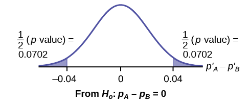
Calculate the p-value using the normal distribution: p\text{-value} = 0.1404.
Estimated proportion for group A: p'_{A} = \dfrac{x_{A}}{n_{A}} = \dfrac{20}{200} = 0.1
Estimated proportion for group B: p'_{B} = \dfrac{x_{B}}{n_{B}} = \dfrac{12}{200} = 0.06
Graph:

Figure 10.4.1.
P′_{A} - P′_{B} = 0.1 – 0.06 = 0.04.
Half the p\text{-value} is below -0.04, and half is above 0.04.
Compare \alpha and the p\text{-value}: \alpha = 0.01 and the p\text{-value} = 0.1404. \alpha < p\text{-value}.
Make a decision: Since \alpha < p\text{-value}, do not reject H_{0}.
Conclusion: At a 1% level of significance, from the sample data, there is not sufficient evidence to conclude that there is a difference in the proportions of adult patients who did not react after 30 minutes to medication A and medication B.
Press STAT. Arrow over to TESTS and press 6:2-PropZTest. Arrow down and enter 20 for x1, 200 for n1, 12 for x2, and 200 for n2. Arrow down to p1: and arrow to not equal p2. Press ENTER. Arrow down to Calculate and press ENTER. The p-value is p = 0.1404 and the test statistic is 1.47. Do the procedure again, but instead of Calculate do Draw.
Exercise \PageIndex{1}
Two types of valves are being tested to determine if there is a difference in pressure tolerances. Fifteen out of a random sample of 100 of Valve A cracked under 4,500 psi. Six out of a random sample of 100 of Valve B cracked under 4,500 psi. Test at a 5% level of significance.
Answer
The p\text{-value} is 0.0379, so we can reject the null hypothesis. At the 5% significance level, the data support that there is a difference in the pressure tolerances between the two valves.
Example \PageIndex{2}: Sexting
A research study was conducted about gender differences in “sexting.” The researcher believed that the proportion of girls involved in “sexting” is less than the proportion of boys involved. The data collected in the spring of 2010 among a random sample of middle and high school students in a large school district in the southern United States is summarized in Table. Is the proportion of girls sending sexts less than the proportion of boys “sexting?” Test at a 1% level of significance.
| Males | Females | |
|---|---|---|
| Sent “sexts” | 183 | 156 |
| Total number surveyed | 2231 | 2169 |
Answer
This is a test of two population proportions. Let M and F be the subscripts for males and females. Then p_{M} and p_{F} are the desired population proportions.
Random variable:p'_{F} - p'_{M} = difference in the proportions of males and females who sent “sexts.”
H_{a}: p_{F} = p_{m} H_{0}: p_{F} - p_{M} = 0
H_{a}: p_{F} < p_{m} H_{a}: p_{F} - p_{M} < 0
The words "less than" tell you the test is left-tailed.
Distribution for the test: Since this is a test of two population proportions, the distribution is normal:
p_{C} = \dfrac{x_{F} + x_{M}}{n_{F} + n_{M}} = \dfrac{156 + 183}{2169 + 2231} = 0.077
1 - p_{C} = 0.923
Therefore,
p'_{F} - p'_{M} \sim N\left(0, \sqrt{(0.077)(0.923)\left(\dfrac{1}{2169} + \dfrac{1}{2231}\right)}\right)
p′_{F} – p′_{M} follows an approximate normal distribution.
Calculate the p\text{-value} using the normal distribution:
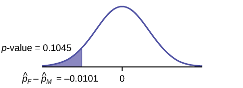
p\text{-value} = 0.1045
Estimated proportion for females: 0.0719
Estimated proportion for males: 0.082
Graph:

Figure 10.4.2.
Decision: Since \alpha < p\text{-value}, Do not reject H_{0}
Conclusion: At the 1% level of significance, from the sample data, there is not sufficient evidence to conclude that the proportion of girls sending “sexts” is less than the proportion of boys sending “sexts.”
Press STAT. Arrow over to TESTS and press 6:2-PropZTest. Arrow down and enter 156 for x1, 2169 for n1, 183 for x2, and 2231 for n2. Arrow down to p1: and arrow to less than p2. Press ENTER. Arrow down to Calculate and press ENTER. The p\text{-value} is P = 0.1045 and the test statistic is z = -1.256.
Example \PageIndex{3}
Researchers conducted a study of smartphone use among adults. A cell phone company claimed that iPhone smartphones are more popular with whites (non-Hispanic) than with African Americans. The results of the survey indicate that of the 232 African American cell phone owners randomly sampled, 5% have an iPhone. Of the 1,343 white cell phone owners randomly sampled, 10% own an iPhone. Test at the 5% level of significance. Is the proportion of white iPhone owners greater than the proportion of African American iPhone owners?
Answer
This is a test of two population proportions. Let W and A be the subscripts for the whites and African Americans. Then pW and pA are the desired population proportions.
Random variable: p′_{W} – p′_{A} = difference in the proportions of Android and iPhone users.
H_{0}: p_{W} = p_{A} H_{0}: p_{W} – p_{A} = 0
H_{a}: p_{W} > p_{A} H_{a}: p_{W} – p_{A} < 0
The words "more popular" indicate that the test is right-tailed.
Distribution for the test: The distribution is approximately normal:
p_{C} = \dfrac{x_{W} + x_{A}}{n_{W} + n_{A}} = \dfrac{134 + 12}{1343 + 232} = 0.0927
1 - p_{C} = 0.9073
Therefore,
p'_{W} - p'_{A} \sim N\left(0, \sqrt{(0.0927)(0.9073)\left(\dfrac{1}{1343} + \dfrac{1}{232}\right)}\right)
p'_{W} - p'_{A} follows an approximate normal distribution.
Calculate the p\text{-value} using the normal distribution:
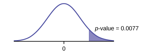
p\text{-value} = 0.0077
Estimated proportion for group A: 0.10
Estimated proportion for group B: 0.05
Graph:

Figure 10.4.3.
Decision: Since \alpha > p\text{-value}, reject the H_{0}.
Conclusion: At the 5% level of significance, from the sample data, there is sufficient evidence to conclude that a larger proportion of white cell phone owners use iPhones than African Americans.
TI-83+ and TI-84: Press STAT. Arrow over to TESTS and press 6:2-PropZTest. Arrow down and enter 135 for x1, 1343 for n1, 12 for x2, and 232 for n2. Arrow down to p1: and arrow to greater than p2. Press ENTER. Arrow down to Calculate and press ENTER. The P-value is P = 0.0092 and the test statistic is Z = 2.33.
Example \PageIndex{3}
A concerned group of citizens wanted to know if the proportion of forcible rapes in Texas was different in 2011 than in 2010. Their research showed that of the 113,231 violent crimes in Texas in 2010, 7,622 of them were forcible rapes. In 2011, 7,439 of the 104,873 violent crimes were in the forcible rape category. Test at a 5% significance level. Answer the following questions:
- Is this a test of two means or two proportions?
- Which distribution do you use to perform the test?
- What is the random variable?
- What are the null and alternative hypothesis? Write the null and alternative hypothesis in symbols.
- Is this test right-, left-, or two-tailed?
- What is the p\text{-value}?
- Do you reject or not reject the null hypothesis?
- At the ___ level of significance, from the sample data, there ______ (is/is not) sufficient evidence to conclude that ____________.
Solutions
a. two proportions
b. normal for two proportions
c. Subscripts: 1 = 2010, 2 = 2011 P′_{1} - P′_{2}
d. Subscripts: 1 = 2010, 2 = 2011 H_{0}: p_{1} = p_{2} H_{0}: p_{1} − p_{2} = 0 H_{0}: p_{1} \neq p_{2} H_{0}: p_{1} − p_{2} \neq 0
e. two-tailed
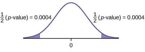
f. p\text{-value} = 0.00086

Figure 10.4.4.
g. Reject the H_{0}.
h. At the 5% significance level, from the sample data, there is sufficient evidence to conclude that there is a difference between the proportion of forcible rapes in 2011 and 2010.
References
- Data from Educational Resources, December catalog.
- Data from Hilton Hotels. Available online at http://www.hilton.com (accessed June 17, 2013).
- Data from Hyatt Hotels. Available online at http://hyatt.com (accessed June 17, 2013).
- Data from Statistics, United States Department of Health and Human Services.
- Data from Whitney Exhibit on loan to San Jose Museum of Art.
- Data from the American Cancer Society. Available online at http://www.cancer.org/index (accessed June 17, 2013).
- Data from the Chancellor’s Office, California Community Colleges, November 1994.
- “State of the States.” Gallup, 2013. Available online at http://www.gallup.com/poll/125066/St...ef=interactive (accessed June 17, 2013).
- “West Nile Virus.” Centers for Disease Control and Prevention. Available online at http://www.cdc.gov/ncidod/dvbid/westnile/index.htm (accessed June 17, 2013).
Chapter Review
- Test of two population proportions from independent samples.
- Random variable: \hat{p}_{A} - \hat{p}_{B} = difference between the two estimated proportions
- Distribution: normal distribution
Formula Review
Pooled Proportion:
p_{c} = \dfrac{x_{F} + x_{M}}{n_{F} + n_{M}}
Distribution for the differences:
p'_{A} - p'_{B} \sim N\left[0, \sqrt{p_{c}(1-p_{c})\left(\dfrac{1}{n_{A}} + \dfrac{1}{n_{B}}\right)}\right]
where the null hypothesis is H_{0}: p_{A} = p_{B} or H_{0}: p_{A} - p_{B} = 0.
Test Statistic (z-score):
z = \dfrac{(p'_{A} - p'_{B})}{\sqrt{p_{c}(1-p_{c})\left(\dfrac{1}{n_{A}} + \dfrac{1}{n_{B}}\right)}}
where the null hypothesis is H_{0}: p_{A} = p_{B} or H_{0}: p_{A} - p_{B} = 0.
and
- p'_{A} and p'_{B} are the sample proportions, p_{A} and p_{B} are the population proportions,
- P_{c} is the pooled proportion, and n_{A} and n_{B} are the sample sizes.
Glossary
- Pooled Proportion
- estimate of the common value of p_{1} and p_{2}.


