
5.8: Applications of Exponential and Logarithmic Functions
- Page ID
- 89911

\( \newcommand{\vecs}[1]{\overset { \scriptstyle \rightharpoonup} {\mathbf{#1}} } \)
\( \newcommand{\vecd}[1]{\overset{-\!-\!\rightharpoonup}{\vphantom{a}\smash {#1}}} \)
\( \newcommand{\dsum}{\displaystyle\sum\limits} \)
\( \newcommand{\dint}{\displaystyle\int\limits} \)
\( \newcommand{\dlim}{\displaystyle\lim\limits} \)
\( \newcommand{\id}{\mathrm{id}}\) \( \newcommand{\Span}{\mathrm{span}}\)
( \newcommand{\kernel}{\mathrm{null}\,}\) \( \newcommand{\range}{\mathrm{range}\,}\)
\( \newcommand{\RealPart}{\mathrm{Re}}\) \( \newcommand{\ImaginaryPart}{\mathrm{Im}}\)
\( \newcommand{\Argument}{\mathrm{Arg}}\) \( \newcommand{\norm}[1]{\| #1 \|}\)
\( \newcommand{\inner}[2]{\langle #1, #2 \rangle}\)
\( \newcommand{\Span}{\mathrm{span}}\)
\( \newcommand{\id}{\mathrm{id}}\)
\( \newcommand{\Span}{\mathrm{span}}\)
\( \newcommand{\kernel}{\mathrm{null}\,}\)
\( \newcommand{\range}{\mathrm{range}\,}\)
\( \newcommand{\RealPart}{\mathrm{Re}}\)
\( \newcommand{\ImaginaryPart}{\mathrm{Im}}\)
\( \newcommand{\Argument}{\mathrm{Arg}}\)
\( \newcommand{\norm}[1]{\| #1 \|}\)
\( \newcommand{\inner}[2]{\langle #1, #2 \rangle}\)
\( \newcommand{\Span}{\mathrm{span}}\) \( \newcommand{\AA}{\unicode[.8,0]{x212B}}\)
\( \newcommand{\vectorA}[1]{\vec{#1}} % arrow\)
\( \newcommand{\vectorAt}[1]{\vec{\text{#1}}} % arrow\)
\( \newcommand{\vectorB}[1]{\overset { \scriptstyle \rightharpoonup} {\mathbf{#1}} } \)
\( \newcommand{\vectorC}[1]{\textbf{#1}} \)
\( \newcommand{\vectorD}[1]{\overrightarrow{#1}} \)
\( \newcommand{\vectorDt}[1]{\overrightarrow{\text{#1}}} \)
\( \newcommand{\vectE}[1]{\overset{-\!-\!\rightharpoonup}{\vphantom{a}\smash{\mathbf {#1}}}} \)
\( \newcommand{\vecs}[1]{\overset { \scriptstyle \rightharpoonup} {\mathbf{#1}} } \)
\(\newcommand{\longvect}{\overrightarrow}\)
\( \newcommand{\vecd}[1]{\overset{-\!-\!\rightharpoonup}{\vphantom{a}\smash {#1}}} \)
\(\newcommand{\avec}{\mathbf a}\) \(\newcommand{\bvec}{\mathbf b}\) \(\newcommand{\cvec}{\mathbf c}\) \(\newcommand{\dvec}{\mathbf d}\) \(\newcommand{\dtil}{\widetilde{\mathbf d}}\) \(\newcommand{\evec}{\mathbf e}\) \(\newcommand{\fvec}{\mathbf f}\) \(\newcommand{\nvec}{\mathbf n}\) \(\newcommand{\pvec}{\mathbf p}\) \(\newcommand{\qvec}{\mathbf q}\) \(\newcommand{\svec}{\mathbf s}\) \(\newcommand{\tvec}{\mathbf t}\) \(\newcommand{\uvec}{\mathbf u}\) \(\newcommand{\vvec}{\mathbf v}\) \(\newcommand{\wvec}{\mathbf w}\) \(\newcommand{\xvec}{\mathbf x}\) \(\newcommand{\yvec}{\mathbf y}\) \(\newcommand{\zvec}{\mathbf z}\) \(\newcommand{\rvec}{\mathbf r}\) \(\newcommand{\mvec}{\mathbf m}\) \(\newcommand{\zerovec}{\mathbf 0}\) \(\newcommand{\onevec}{\mathbf 1}\) \(\newcommand{\real}{\mathbb R}\) \(\newcommand{\twovec}[2]{\left[\begin{array}{r}#1 \\ #2 \end{array}\right]}\) \(\newcommand{\ctwovec}[2]{\left[\begin{array}{c}#1 \\ #2 \end{array}\right]}\) \(\newcommand{\threevec}[3]{\left[\begin{array}{r}#1 \\ #2 \\ #3 \end{array}\right]}\) \(\newcommand{\cthreevec}[3]{\left[\begin{array}{c}#1 \\ #2 \\ #3 \end{array}\right]}\) \(\newcommand{\fourvec}[4]{\left[\begin{array}{r}#1 \\ #2 \\ #3 \\ #4 \end{array}\right]}\) \(\newcommand{\cfourvec}[4]{\left[\begin{array}{c}#1 \\ #2 \\ #3 \\ #4 \end{array}\right]}\) \(\newcommand{\fivevec}[5]{\left[\begin{array}{r}#1 \\ #2 \\ #3 \\ #4 \\ #5 \\ \end{array}\right]}\) \(\newcommand{\cfivevec}[5]{\left[\begin{array}{c}#1 \\ #2 \\ #3 \\ #4 \\ #5 \\ \end{array}\right]}\) \(\newcommand{\mattwo}[4]{\left[\begin{array}{rr}#1 \amp #2 \\ #3 \amp #4 \\ \end{array}\right]}\) \(\newcommand{\laspan}[1]{\text{Span}\{#1\}}\) \(\newcommand{\bcal}{\cal B}\) \(\newcommand{\ccal}{\cal C}\) \(\newcommand{\scal}{\cal S}\) \(\newcommand{\wcal}{\cal W}\) \(\newcommand{\ecal}{\cal E}\) \(\newcommand{\coords}[2]{\left\{#1\right\}_{#2}}\) \(\newcommand{\gray}[1]{\color{gray}{#1}}\) \(\newcommand{\lgray}[1]{\color{lightgray}{#1}}\) \(\newcommand{\rank}{\operatorname{rank}}\) \(\newcommand{\row}{\text{Row}}\) \(\newcommand{\col}{\text{Col}}\) \(\renewcommand{\row}{\text{Row}}\) \(\newcommand{\nul}{\text{Nul}}\) \(\newcommand{\var}{\text{Var}}\) \(\newcommand{\corr}{\text{corr}}\) \(\newcommand{\len}[1]{\left|#1\right|}\) \(\newcommand{\bbar}{\overline{\bvec}}\) \(\newcommand{\bhat}{\widehat{\bvec}}\) \(\newcommand{\bperp}{\bvec^\perp}\) \(\newcommand{\xhat}{\widehat{\xvec}}\) \(\newcommand{\vhat}{\widehat{\vvec}}\) \(\newcommand{\uhat}{\widehat{\uvec}}\) \(\newcommand{\what}{\widehat{\wvec}}\) \(\newcommand{\Sighat}{\widehat{\Sigma}}\) \(\newcommand{\lt}{<}\) \(\newcommand{\gt}{>}\) \(\newcommand{\amp}{&}\) \(\definecolor{fillinmathshade}{gray}{0.9}\)- Apply common exponential models to real-life situations.
- Apply common logarithmic models to real-life situations.
We have already explored some basic applications of exponential and logarithmic functions. In this section, we explore some important applications in more depth, including radioactive isotopes and Newton’s Law of Cooling.
Modeling Exponential Growth and Decay
In real-world applications, we need to model the behavior with functions. In mathematical modeling, we choose a familiar general function with properties that suggest that it will model the real-world phenomenon we wish to analyze. In the case of population growth, such as a bacteria culture that a biologist is studying for a new medical treatment, we may choose the exponential growth function:
\[N(t)=N_0e^{rt}\nonumber\]
where \(N_0\) is equal to the value at time zero, \(e\) is Euler’s constant, and \(k\) is a positive constant that determines the rate (percentage) of growth.
The model \(N(t)=N_0\cdot e^{kt}\) represents the population size after a given amount of time \(t\).
\(N_0\) is the initial population size and \(r\) is the rate of growth for the population.
A population of bacteria doubles in size every hour. If the culture started with \(10\) bacteria, find a model that describes the population size after of the bacteria after \(t\) hours. Use this model to determine how many bacteria there will be after 10 hours.
Solution
Bacteria growth is exponential. To find \(N_0\) we use the fact that \(N_0\) is the amount at time zero, so \(N_0=10\). To find \(r\), use the fact that after one hour \((t=1)\) the population doubles from \(10\) to \(20\). The formula is derived as follows
\[\begin{align*} 20&= 10e^{r\cdot 1}\\ 2&= e^r \qquad \text{Divide by 10}\\ \ln2&= r \qquad \text{Convert to exponential form} \end{align*}\]
so \(r=\ln(2)\). Thus the equation that models the bacteria growth is \(N(t)=10e^{(\ln2)t}=10{(e^{\ln2})}^t=10·2^t\). The graph is shown in Figure \(\PageIndex{2}\).
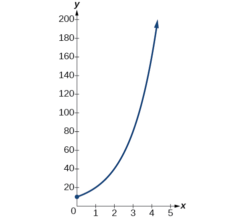
The population of bacteria after ten hours is \(N(10)=10\cdot2^10=10,240\).
Analysis
We could describe this amount is being of the order of magnitude \(10^4\). The population of bacteria after twenty hours is \(10,485,760\) which is of the order of magnitude \(10^7\), so we could say that the population has increased by three orders of magnitude in ten hours.
In the previous example, we were provided information about the time it took for the population to double in size. This time is called doubling time. Notice that the model simplified to an exponential function of base 2. We can describe a modified growth model for doubling time as follows:
The model \(N(t)=N_0\cdot2^{\frac{t}{d}}\) represents the population size after a given amount of time \(t\).
\(N_0\) is the initial population size and \(a\) is the time it takes for the population to double in size.
Cancer cells sometimes increase exponentially. If a cancerous growth contained 300 cells last month and 360 cells this month, how long will it take for the number of cancer cells to double? Round your answer to the nearest tenth.
Solution
Defining \(t\) to be time in months, with \(t = 0\) corresponding to the initial size of the population, we are given two pieces of data: last month, (0, 300) and this month, (1, 360).
From this data, we can find an equation for the growth. Using the form \(N(t)=N_0\cdot2^{\frac{t}{d}}\), we know immediately \(N_0=300\), giving \(N(t)=300\cdot2^{t}\). Substituting in \((1,360)\), \[\begin{align*} 360&=300\cdot2^\tfrac{1}{d} \\[4pt] \dfrac{360}{300}&= 2^\tfrac{1}{d}\\[4pt] 1.2&= 2^\tfrac{1}{d} \\[4pt] \ln1.2&=\ln\left(2^{\tfrac{1}{d}}\right) \\[4pt] \ln1.2&=\dfrac{1}{d}\ln2 \\[4pt] d\cdot\ln1.2&=\ln2 \\[4pt] d&=\dfrac{\ln2}{\ln1.2} \\[4pt] d &\approx3.8 \text{ months}\end{align*}\nonumber\]
Radioactive Decay and Half-Life
We now turn to exponential decay. One of the common terms associated with exponential decay is half-life, the length of time it takes an exponentially decaying quantity to decrease to half its original amount. Every radioactive isotope has a half-life, and the process describing the exponential decay of an isotope is called radioactive decay.
The model \(M(t)=M_0e^{-\tfrac{ln2}{h}t}\) represents the amount of material (mass) left after a given amount of time \(t\).
\(M_0\) is the initial mass size and \(h\) is the half-life of the material.
The formula for radioactive decay is important in radiocarbon dating, which is used to calculate the approximate date a plant or animal died. Radiocarbon dating was discovered in 1949 by Willard Libby, who won a Nobel Prize for his discovery. It compares the difference between the ratio of two isotopes of carbon in an organic artifact or fossil to the ratio of those two isotopes in the air. It is believed to be accurate to within about \(1\%\) error for plants or animals that died within the last \(60,000\) years.
Carbon-14 is a radioactive isotope of carbon that has a half-life of \(5,730\) years. It occurs in small quantities in the carbon dioxide in the air we breathe. Most of the carbon on Earth is carbon-12, which has an atomic weight of \(12\) and is not radioactive. Scientists have determined the ratio of carbon-14 to carbon-12 in the air for the last \(60,000\) years, using tree rings and other organic samples of known dates—although the ratio has changed slightly over the centuries.
As long as a plant or animal is alive, the ratio of the two isotopes of carbon in its body is close to the ratio in the atmosphere. When it dies, the carbon-14 in its body decays and is not replaced. By comparing the ratio of carbon-14 to carbon-12 in a decaying sample to the known ratio in the atmosphere, the date the plant or animal died can be approximated.
The half-life of carbon-14 is \(5,730\) years. Express the amount of carbon-14 remaining as a function of time, \(t\).
Solution
The function that describes this continuous decay is \(M(t)=M_0e^{\left (-\tfrac{\ln(2)}{5730} \right )t}\).
A bone fragment is found that contains \(20\%\) of its original carbon-14. To the nearest year, how old is the bone?
Solution
The percentage of carbon-14 in all living things is \(100\%\). The percentage of carbon-14 after some amount of time, \(t\), (which we are trying to find) is 20%. Using decimals for the percent, we can substitute in \(M_0=1 \text{ and } M(t)=0.2\) into the function we found in the previous example, \[\begin{align*}M(t)&=M_0e^{\left (-\tfrac{\ln(2)}{5730} \right )t}\\[4pt] 0.2&=1\cdot e^{\left (-\tfrac{\ln(2)}{5730} \right )t} \\[4pt] 0.2&=e^{\left (-\tfrac{\ln(2)}{5730} \right )t} \\[4pt] \ln0.2&=\frac{-\ln(2)}{5730}t\\[4pt] -\dfrac{5730}{\ln2}(\ln0.2)&=t\\[4pt] t &\approx13,305 \text{ years}\end{align*}\]
The bone fragment is about \(13,305\) years old.
Analysis
The instruments that measure the percentage of carbon-14 are extremely sensitive and, as we mention above, a scientist will need to do much more work than we did in order to be satisfied. Even so, carbon dating is only accurate to about \(1\%\), so this age should be given as \(13,305\) years \(\pm 1\%\) or \(13,305\) years \(\pm 133\) years.
Newton’s Law of Cooling
Exponential decay can also be applied to temperature. When a hot object is left in surrounding air that is at a lower temperature, the object’s temperature will decrease exponentially, leveling off as it approaches the surrounding air temperature. On a graph of the temperature function, the leveling off will correspond to a horizontal asymptote at the temperature of the surrounding air. Unless the room temperature is zero, this will correspond to a vertical shift of the generic exponential decay function. This translation leads to Newton’s Law of Cooling, the scientific formula for temperature as a function of time as an object’s temperature is equalized with the ambient temperature
The temperature of an object, \(T\), in surrounding air with temperature \(T_s\) will behave according to the formula
\[T(t)=D_0e^{-kt}+T_s\nonumber\]
where- \(t\) is time
- \(D_0\) is the difference between the initial temperature of the object and the surroundings
- \(k\) is a constant, the continuous rate of cooling of the object
A cheesecake is taken out of the oven with an ideal internal temperature of \(165°F\), and is placed into a \(35°F\) refrigerator. After \(10\) minutes, the cheesecake has cooled to \(150°F\). If we must wait until the cheesecake has cooled to \(70°F\) before we eat it, how long will we have to wait?
Solution
Because the surrounding air temperature in the refrigerator is \(35\) degrees, the cheesecake’s temperature will decay exponentially toward \(35\), following the equation
\(T(t)=D_0e^{-kt}+35\)
We know the initial temperature was \(165\), so \(T(0)=165\).
\[\begin{align*} 165&= Ae^{-k0}+35 \qquad \text{Substitute } (0,165)\\ D_0&= 130 \qquad \text{Solve for } D_0 \end{align*}\]
We were given another data point, \(T(10)=150\), which we can use to solve for \(k\).
\[\begin{align*} 150&= 130e^{-k10}+35 \qquad \text{Substitute } (10, 150)\\ 115&= 130e^{-k10} \qquad \text{Subtract 35}\\ \dfrac{115}{130}&= e^{-10k} \qquad \text{Divide by 130}\\ \ln\left (\dfrac{115}{130} \right )&= -10k \qquad \text{Take the natural log of both sides}\\ k &= \dfrac{\ln \left (\dfrac{115}{130} \right )}{-10} \qquad \text{Divide by the coefficient of k} \end{align*}\]
This gives us the equation for the cooling of the cheesecake: \(T(t)=130e^{\left(–\tfrac{1}{10} \ln\tfrac{23}{26}t \right)}+35\).
Now we can solve for the time it will take for the temperature to cool to \(70\) degrees. \[\begin{align*} 70&= 130e^{\left(–\tfrac{1}{10} \ln\tfrac{23}{26} \right)}+35 \qquad \text{Substitute in 70 for } T(t)\\[4pt]
35&= 130e^{\left(–\tfrac{1}{10} \ln\tfrac{23}{26} \right)t} \qquad \text{Subtract 35}\\[4pt]
\dfrac{35}{130}&= e^{\left(–\tfrac{1}{10} \ln\tfrac{23}{26} \right)t} \qquad \text{Divide by 130}\\[4pt]
\ln \left (\dfrac{35}{130} \right )&= \left(–\tfrac{1}{10} \ln\tfrac{23}{26} \right)t \qquad \text{Take the natural log of both sides}\\[4pt]
t&= \dfrac{\ln \left (\dfrac{35}{130} \right )}{\left(–\tfrac{1}{10} \ln\tfrac{23}{26} \right)t}\\[4pt]
t&\approx 107 \qquad \text{Divide by the coefficient of t} \end{align*}\]
It will take about \(107\) minutes, or one hour and \(47\) minutes, for the cheesecake to cool to \(70°F\).
A pitcher of water at \(40\) degrees Fahrenheit is placed into a \(70\) degree room. One hour later, the temperature has risen to \(45\) degrees. How long will it take for the temperature to rise to \(60\) degrees to three decimal places?
- Answer
-
\(6.026\) hours
Modeling with Logarithms
For quantities that vary greatly in magnitude, a standard scale of measurement is not always effective, and utilizing logarithms can make the values more manageable. For example, if the average distances from the sun to the major bodies in our solar system are listed, you see they vary greatly.
| Planet | Distance (millions of km) |
| Mercury | 58 |
| Venus | 108 |
| Earth | 150 |
| Mars | 228 |
| Jupiter | 779 |
| Saturn | 1430 |
| Uranus | 2880 |
| Neptune | 4500 |
Placed on a linear scale – one with equally spaced values – these values get bunched up, as seen below.
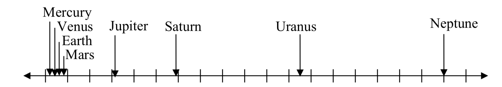
0 500 1000 1500 2000 2500 3000 3500 4000 4500
However, computing the logarithm of each value and plotting these new values on a number line results in a more manageable graph, and makes the relative distances more apparent.
| Planet | Distance (millions of km) | log(distance) |
| Mercury | 58 | 1.76 |
| Venus | 108 | 2.03 |
| Earth | 150 | 2.18 |
| Mars | 228 | 2.36 |
| Jupiter | 779 | 2.89 |
| Saturn | 1430 | 3.16 |
| Uranus | 2880 | 3.46 |
| Neptune | 4500 | 3.65 |
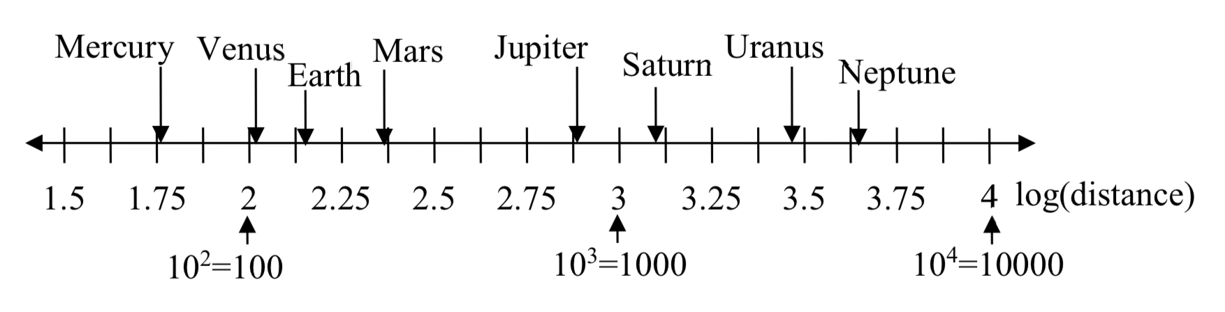
(It is interesting to note the large gap between Mars and Jupiter on the log number line. There is an asteroid belt located there, which some scientists believe is a planet that never formed because of the effects of the gravity of Jupiter.)
Logarithms are also used to measure sound intensity levels.
| Source of Sound/Noise | Approximate Sound Pressure in \(\mu\) Pa (micro Pascals) |
| Launching of the Space Shuttle | 2000,000,000 |
| Full Symphony Orchestra | 2000,000 |
| Diesel Freight Train at High Speed at 25 m | 200,000 |
| Normal Conversation | 20,000 |
| Soft Whispering at 2 m in Library | 2,000 |
| Unoccupied Broadcast Studio Room | 200 |
| Softest Sound a human can hear | 20 |
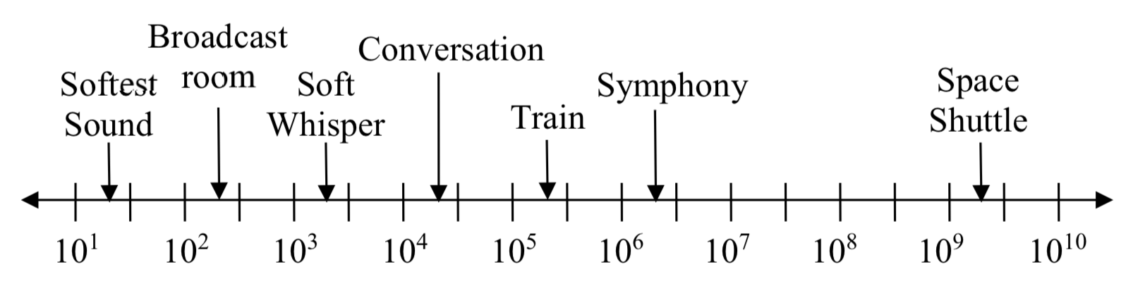
Logarithms are useful for showing relative changes. For example, comparing the sound of a diesel freight train to a soft whisper, the diesel train is 100 times larger than a soft whisper.
\[\dfrac{200,000}{2,000} = 100 = 10^2\nonumber\]
When one quantity is roughly ten times larger than another, we say it is one order of magnitude larger. The order of magnitude can be found as the common logarithm of the ratio of the quantities.
Given two values \(A\) and \(B\), to determine how many orders of magnitude \(A\) is greater than \(B\),
Difference in orders of magnitude = log(\(\dfrac{A}{B})\)
One example of a logarithmic scale is the Moment Magnitude Scale (MMS) used for earthquakes. This scale is commonly and mistakenly called the Richter Scale, which was a very similar scale succeeded by the MMS.
For an earthquake with seismic moment \(S\), a measurement of earth movement, the MMS value, or magnitude \(M\) of an earthquake, is
\[M = \dfrac{2}{3} log(\dfrac{S}{S_0})\nonumber\]
Where \(S_0 = 10^{16}\) is a baseline measure for the seismic moment.
If one earthquake has a MMS magnitude of 6.0, and another has a magnitude of 8.0, how much more powerful (in terms of earth movement) is the second earthquake?
Solution
Since the first earthquake has magnitude 6.0, we can find the amount of earth movement for that quake, which we'll denote \(S_1\). The value of \(S_0\) is not particularity relevant, so we will not replace it with its value.
\[6.0 = \dfrac{2}{3} log \left(\dfrac{S_1}{S_0}\right)\nonumber\]
\[6.0 \left(\dfrac{3}{2}\right) = log \left(\dfrac{S_1}{S_0}\right)\nonumber\]
\[9 = log\left(\dfrac{S_1}{S_0}\right)\nonumber\]
\[\dfrac{S_1}{S_0} = 10^9\nonumber\]
\[S_1 = 10^9 S_0\nonumber\]
This tells us the first earthquake has about \(10^9\) times more earth movement than the baseline measure, \(S_0\).
Doing the same with the second earthquake, \(S_2\), with a magnitude of 8.0,
\[8.0 = \dfrac{2}{3} log \left(\dfrac{S_2}{S_0}\right)\nonumber\]
\[S_2 = 10^{12} S_0\nonumber\]
Comparing the earth movement of the second earthquake to the first,
\[\dfrac{S_2}{S_1} = \dfrac{10^{12} S_0} {10^9 S_0} = 10^3 = 1000\nonumber\]
The second value's earth movement is 1000 times as large as the first earthquake.
One earthquake has magnitude of 3.0. If a second earthquake has twice as much earth movement as the first earthquake, find the magnitude of the second quake.
Solution
Since the first quake has magnitude 3.0,
\[3.0 = \dfrac{2}{3} log (\dfrac{S}{S_0})\nonumber\]
Solving for \(S\),
\[3.0 \dfrac{3}{2} = log (\dfrac{S}{S_0})\nonumber\]
\[4.5 = log (\dfrac{S}{S_0})\nonumber\]
\[10^{4.5} = \dfrac{S}{S_0}\nonumber\]
\[S = 10^{4.5} S_0\nonumber\]
Since the second earthquake has twice as much earth movement, for the second quake,
\[S = 2 \cdot 10^{4.5} S_0\nonumber\]
Finding the magnitude,
\[M = \dfrac{2}{3} log (\dfrac{2 \cdot 10^{4.5} S_0}{S_0})\nonumber\]
\[M = \dfrac{2}{3} log (2 \cdot 10^{4.5}) \approx 3.201\nonumber\]
The second earthquake with twice as much earth movement will have a magnitude of about 3.2.
As we saw in an earlier section, logarithms are also used to describe \(pH\) levels.
The pH of a solutions is defined by the following formula, where \([\ce{H^{+}}]\) is the concentration of hydrogen ions in the solution
\[\begin{align*} {pH}&=−{\log}([\ce{H^{+}}]) \label{eq1} \\[4pt] &={\log}\left(\dfrac{1}{[\ce{H^{+}}]}\right) \label{eq2} \end{align*}\nonumber\]
If the concentration of hydrogen ions in a liquid is doubled, what is the effect on pH?
Solution
Suppose \(C\) is the original concentration of hydrogen ions, and \(P\) is the original pH of the liquid. Then \(P=–\log(C)\). If the concentration is doubled, the new concentration is \(2C\). Then the pH of the new liquid is
\(pH=−\log(2C)\)
Using the product rule of logs
\(pH=−\log(2C)=−(\log(2)+\log(C))=−\log(2)−\log(C)\)
Since \(P=–\log(C)\),the new pH is
\(pH=P−\log(2)≈P−0.301\)