4.2: Polynomial Functions

In the previous section we explored the short run behavior of quadratics, a special case of polynomials.  In this section we will explore the behavior of polynomials in general.  The basic building blocks of polynomials are power functions.

Definition: Power Function

A power function is a function that can be represented in the form

\[f(x)=x^p \label{power}\]

where the base is the variable and the exponent, \(p\), is a numbers.

Q&A: Is \(f(x)=2^x\) a power function?

No. A power function contains a variable base raised to a fixed power (Equation \ref{power}). This function has a constant base raised to a variable power. This is called an exponential function, not a power function. This function will be discussed later.

Characteristics of Power Functions

Figure \(\PageIndex{2}\) shows the graphs of \(f(x)=x^2\), \(g(x)=x^4\) and and \(h(x)=x^6\), which are all power functions with even, whole-number powers. Notice that these graphs have similar shapes, very much like that of the quadratic function in the toolkit. However, as the power increases, the graphs flatten somewhat near the origin and become steeper away from the origin.

Figure \(\PageIndex{2}\): Even-power functions

To describe the behavior as numbers become larger and larger, we use the idea of infinity. We use the symbol \(\infty\) for positive infinity and \(−\infty\) for negative infinity. When we say that “x approaches infinity,” which can be symbolically written as \(x{\rightarrow}\infty\), we are describing a behavior; we are saying that \(x\) is increasing without bound.

With the even-power function, as the input increases or decreases without bound, the output values become very large, positive numbers. Equivalently, we could describe this behavior by saying that as \(x\) approaches positive or negative infinity, the \(f(x)\) values increase without bound. In symbolic form, we could write

\[\text{as } x{\rightarrow}{\pm}{\infty}, \;f(x){\rightarrow}{\infty} \nonumber\]

Figure \(\PageIndex{3}\) shows the graphs of \(f(x)=x^3\), \(g(x)=x^5\), and \(h(x)=x^7\), which are all power functions with odd, whole-number powers. Notice that these graphs look similar to the cubic function in the toolkit. Again, as the power increases, the graphs flatten near the origin and become steeper away from the origin.

Figure \(\PageIndex{3}\): Odd-power function

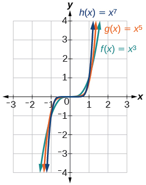
These examples illustrate that functions of the form \(f(x)=x^n\) reveal symmetry of one kind or another. First, in Figure \(\PageIndex{2}\) we see that even functions of the form \(f(x)=x^n\), \(n\) even, are symmetric about the \(y\)-axis. In Figure \(\PageIndex{3}\) we see that odd functions of the form \(f(x)=x^n\), \(n\) odd, are symmetric about the origin.

For these odd power functions, as \(x\) approaches negative infinity, \(f(x)\) decreases without bound. As \(x\) approaches positive infinity, \(f(x)\) increases without bound. In symbolic form we write

\[\begin{align*} &\text{as }x{\rightarrow}-{\infty},\;f(x){\rightarrow}-{\infty} \\ &\text{as }x{\rightarrow}{\infty},\;f(x){\rightarrow}{\infty} \end{align*}\]

Long Run Behavior

The behavior of the graph of a function as the input values get very small \((x{\rightarrow}−{\infty})\) and get very large \(x{\rightarrow}{\infty}\) is referred to as the long run behavior of the function. We can use words or symbols to describe end behavior.

Polynomials

Definition: Word

A polynomial is function that can be written as \(f(x) = {a_0} + {a_1}x + {a_2}{x^2} +  \cdots  + {a_n}{x^n}\)

Each of the a_i constants are called coefficients and can be positive, negative, or zero, and be whole numbers, decimals, or fractions.

A term of the polynomial is any one piece of the sum, that is any \(a_ix^i\). Each individual term is a transformed power function.

The degree of the polynomial is the highest power of the variable that occurs in the polynomial.

The leading term is the term containing the highest power of the variable: the term with the highest degree.

The leading coefficient is the coefficient of the leading term.

Because of the definition of the “leading” term we often rearrange polynomials so that the powers are descending. \(f(x) = {a_n}{x^n} + ..... + {a_2}{x^2} + {a_1}x + a_0\)

Example \(\PageIndex{1}\)

Which of the following are polynomial functions?

• \(f(x)=2x^3⋅3x+4\)
• \(g(x)=−x(x^2−4)\)
• \(h(x)=5\sqrt{x}+2\)

Solution

For the function \(f(x)\), the degree is 3, the highest power on \(x\).  The leading term is the term containing that power, \(- 4x^3\).  The leading coefficient is the coefficient of that term, -4.

For \(g(t)\), the degree is 5, the leading term is \(5{t^5}\), and the leading coefficient is 5.

Example \(\PageIndex{1}\): Identifying the Degree and Leading Coefficient of a Polynomial Function

Identify the degree, leading term, and leading coefficient of the following polynomial functions.

\(f(x)=3+2x^2−4x^3\)

\(g(t)=5t^5−2t^3+7t\)

\(h(p)=6p−p^3−2\)

Solution

For the function \(f(x)\), the highest power of \(x\) is 3, so the degree is 3. The leading term is the term containing that degree, \(−4x^3\). The leading coefficient is the coefficient of that term, −4.

For the function \(g(t)\), the highest power of \(t\) is 5, so the degree is 5. The leading term is the term containing that degree, \(5t^5\). The leading coefficient is the coefficient of that term, 5.

For the function \(h(p)\), the highest power of \(p\) is 3, so the degree is 3. The leading term is the term containing that degree, \(−p^3\); the leading coefficient is the coefficient of that term, −1.

Long Run Behavior of Polynomials

For any polynomial, the long run behavior of the polynomial will match the long run behavior of the leading term.

Example \(\PageIndex{2}\): Identifying End Behavior and Degree of a Polynomial Function

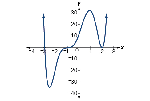
What can we determine about the long run behavior and degree of the equation for the polynomial graphed in Figure \(\PageIndex{8}\).

Figure \(\PageIndex{8}\).

Solution

Since the output grows large and positive as the inputs grow large and positive, we describe the long run behavior symbolically by writing:

\[\text{as } x{\rightarrow}{\infty}, \; f(x){\rightarrow}{\infty} \nonumber\]

\[\text{as } x{\rightarrow}-{\infty}, \; f(x){\rightarrow}-{\infty} \nonumber\]

In words, we could say that as \(x\) values approach infinity, the function values approach infinity, and as \(x\) values approach negative infinity, the function values approach negative infinity.

We can tell this graph has the shape of an odd degree power function that has not been reflected, so the degree of the polynomial creating this graph must be odd and the leading coefficient must be positive.

Short Run Behavior: Intercepts

Characteristics of the graph such as vertical and horizontal intercepts and the places the graph changes direction are part of the short run behavior of the polynomial. 

Like with all functions, the vertical intercept is where the graph crosses the vertical axis, and occurs when the input value is zero.  Since a polynomial is a function, there can only be one vertical intercept, which occurs at the point \(0, a_0\).  The horizontal intercepts occur at the input values that correspond with an output value of zero.  It is possible to have more than one horizontal intercept.

Horizontal intercepts are also called zeros, or roots of the function.

To find horizontal intercepts, we need to solve for when the output will be zero.  For general polynomials, this can be a challenging prospect.  While quadratics can be solved using the relatively simple quadratic formula, the corresponding formulas for cubic and 4^th degree polynomials are not simple enough to remember, and formulas do not exist for general higher-degree polynomials.  Consequently, we will limit ourselves to three cases:

1. The polynomial can be factored using known methods: greatest common factor and trinomial factoring. 
2. The polynomial is given in factored form.
3. Technology is used to determine the intercepts.

Example \(\PageIndex{3}\)

Find the horizontal intercepts of \(f(x) = {x^6} - 3{x^4} + 2{x^2}\).

Solution

We can attempt to factor this polynomial to find solutions for \(f(x) = 0\).

\[\begin{align*}
x^6- 3x^4 + 2x^2&= 0\quad && \text{Factoring out the greatest common factor}\\
x^2\left( x^4 - 3x^2 + 2\right) &= 0\quad &&    \text{Factoring the inside as a quadratic in $x^2$} \\
x^2\left( x^2- 1\right)\left(x^2 - 2\right) &= 0\quad &&   \text{Then break apart to find solutions}\\
x^2 = 0 \quad & \quad \left(x^2 - 1\right) = 0  &&\quad \left(x^2-2\right)\\
x = 0 \quad &\quad \; x^2= 1&&\quad\;  x^2=2 \\
&\quad \; x =\pm \sqrt 2 &&\;\quad x=\pm\sqrt{2}
\end{align*} \]This gives us 5 horizontal intercepts.

Example \(\PageIndex{4}\)

Find the vertical and horizontal intercepts of \(g(t) = (t - 2)^2(2t + 3)\).

Solution

The vertical intercept can be found by evaluating \(g(0)\). 

\(g(0) = {(0 - 2)^2}(2(0) + 3) = 12\)

The horizontal intercepts can be found by solving \(g(t) = 0\).

\[(t - 2)^2(2t + 3) = 0 \nonumber\]

Since this is already factored, we can break it apart:

\[\begin{align*}
(t - 2)^2&= 0 \quad\quad& (2t + 3)&= 0 \\
t - 2 &= 0 \quad&t &= \frac{- 3}{2} \\
t &= 2&&
\end{align*} \]

Example \(\PageIndex{5}\)

Find the horizontal intercepts of \(h(t) = {t^3} + 4{t^2} + t - 6\)

Solution

Since this polynomial is not in factored form, has no common factors, and does not appear to be factorable using techniques we know, we can turn to technology to find the intercepts. 

Graphing this function, it appears there are horizontal intercepts at \(t = -3, -2\), and \(1\).

We could check these are correct by plugging in these values for t and verifying that \(h( - 3) = h( - 2) = h(1) = 0\).

Notice that the polynomial in the previous example was degree three, and had three horizontal intercepts and two turning points – places where the graph changes direction.  We will now make a general statement without justifying it.

Definition: Intercepts and Turning Points of Polynomials

A polynomial of degree n will have:

At most \(n\) horizontal intercepts.  An odd degree polynomial will always have at least one,

At most \(n-1\) turning points.

Exercise \(\PageIndex{1}\)

Find the vertical and horizontal intercepts of the function \(f(t)=t^4-4t^2\).

Answer

Vertical intercept \((0, 0)\), Horizontal intercepts \((0, 0)\), \((-2, 0)\), \((2, 0)\)

Graphical Behavior at Intercepts

If we graph the function \(f(x)=(x+3)(x−2)^2(x+1)^3,\) notice that the behavior at each of the horizontal intercepts is different.

Figure \(\PageIndex{7}\): Identifying the behavior of the graph at an horizontal intercept by examining the multiplicity of the zero.

The horizontal intercept \(x=−3\), coming from the \((x+3)\) factor of the polynomial, the graph passes directly through the horizontal intercept.  The factor is linear (has a power of 1), so the behavior near the intercept is like that of a line - it passes directly through the intercept. We call this a single zero, since the zero corresponds to a single factor of the function.

At the horizontal intercept \(x=2\) coming from the \((x−2)^2\) factor of the polynomial, the graph touches the axis at the intercept and changes direction.  The factor is quadratic (degree 2), so the behavior near the intercept is like that of a quadratic – it bounces off of the horizontal axis at the intercept.  Since 

\[(x−2)^2=(x−2)(x−2), \nonumber\]

The factor is repeated twice, that is, the factor \((x−2)\) appears twice, so we call this a double zero. We could also say the zero has multiplicity 2.

The horizontal intercept \(x=−1\) coming from the  \((x+1)^3\) factor of the polynomial, the graph passes through the axis at the intercept, but flattens out a bit first.  This factor is cubic (degree 3), so the behavior near the intercept is like that of a cubic, with the same “S” type shape near the intercept that the toolkit \(x^3\) has. We call this a triple zero. We could also say the zero has multiplicity 3.

By utilizing these behaviors, we can sketch a reasonable graph of a factored polynomial function without needing technology.

Graphical Behavior of Polynomials at Horizontal Intercepts

If a polynomial contains a factor of the form \((x-h)^p\), the behavior near the horizontal intercept h is determined by the power on the factor.

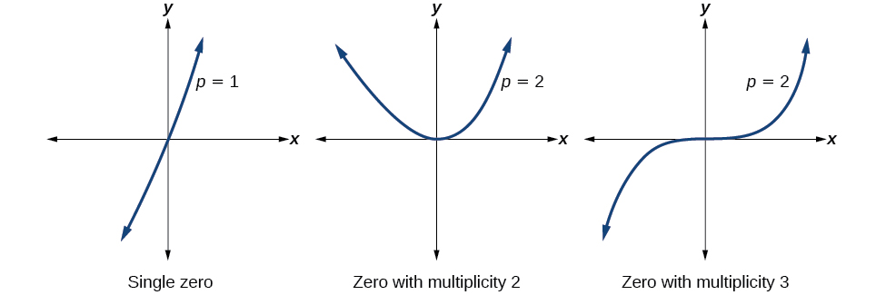Figure \(\PageIndex{8}\): Three graphs showing three different polynomial functions with multiplicity 1, 2, and 3.

For higher even powers 4, 6, 8 etc.… the graph will still bounce off of the horizontal axis but the graph will appear flatter with each increasing even power as it approaches and leaves the axis.

For higher odd powers, 5, 7, 9 etc… the graph will still pass through the horizontal axis but the graph will appear flatter with each increasing odd power as it approaches and leaves the axis.

Example \(\PageIndex{8}\): Sketching the Graph of a Polynomial Function

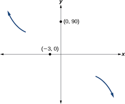
Sketch a graph of \(f(x)=−2(x+3)^2(x−5)\).

Solution

This graph has two x-intercepts. At \(x=−3\), the factor is squared, indicating a multiplicity of 2. The graph will bounce at this x-intercept. At \(x=5\),the function has a multiplicity of one, indicating the graph will cross through the axis at this intercept.

The y-intercept is found by evaluating \(f(0)\).

\[\begin{align*} f(0)&=−2(0+3)^2(0−5) \\ &=−2⋅9⋅(−5) \\ &=90 \end{align*}\]

The y-intercept is \((0,90)\).

Additionally, we can see the leading term, if this polynomial were multiplied out, would be \(−2x3\), so the end behavior is that of a vertically reflected cubic, with the outputs decreasing as the inputs approach infinity, and the outputs increasing as the inputs approach negative infinity. See Figure \(\PageIndex{13}\).

Figure \(\PageIndex{13}\): Showing the distribution for the leading term.

To sketch this, we consider that:

• As \(x{\rightarrow}−{\infty}\) the function \(f(x){\rightarrow}{\infty}\),so we know the graph starts in the second quadrant and is decreasing toward the x-axis.
• Since \(f(−x)=−2(−x+3)^2(−x–5)\) is not equal to \(f(x)\), the graph does not display symmetry.
• At \((−3,0)\), the graph bounces off of thex-axis, so the function must start increasing.
• At \((0,90)\), the graph crosses the y-axis at the y-intercept. See Figure \(\PageIndex{14}\).

Figure \(\PageIndex{14}\): Graph of the end behavior and intercepts, \((-3, 0)\) and \((0, 90)\), for the function \(f(x)=-2(x+3)^2(x-5)\).

Somewhere after this point, the graph must turn back down or start decreasing toward the horizontal axis because the graph passes through the next intercept at \((5,0)\). See Figure \(\PageIndex{15}\).

Figure \(\PageIndex{15}\): Graph of the end behavior and intercepts, \((-3, 0)\), \((0, 90)\) and \((5, 0)\), for the function \(f(x)=-2(x+3)^2(x-5)\).

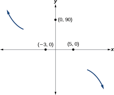
As \(x{\rightarrow}{\infty}\) the function \(f(x){\rightarrow}−{\infty}\),

so we know the graph continues to decrease, and we can stop drawing the graph in the fourth quadrant.

Using technology, we can create the graph for the polynomial function, shown in Figure \(\PageIndex{16}\), and verify that the resulting graph looks like our sketch in Figure \(\PageIndex{15}\).

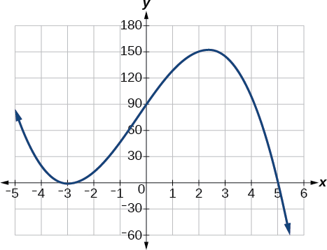
Figure \(\PageIndex{16}\): The complete graph of the polynomial function \(f(x)=−2(x+3)^2(x−5)\).

Solving Polynomial Inequalities

One application of our ability to find intercepts and sketch a graph of polynomials is the ability to solve polynomial inequalities.  It is a very common question to ask when a function will be positive and negative.  We can solve polynomial inequalities by either utilizing the graph, or by using test values.

Example \(\PageIndex{7}\)

Solve \((x + 3)(x + 1)^2(x - 4) > 0\).

Solution

As with all inequalities, we start by solving the equality \((x + 3)(x + 1)^2(x - 4) = 0\), which has solutions at \(x= -3, -1,\) and \(4\).  We know the function can only change from positive to negative at these values, so these divide the inputs into 4 intervals. 

We could choose a test value in each interval and evaluate the function \(f(x) = (x + 3){(x + 1)^2}(x - 4)\) at each test value to determine if the function is positive or negative in that interval

Interval	Test \(x\) in interval	\(f\)(test value)	>0 or <0?
\(x < -3\)	-4	72	> 0
\(-3 < x < -1\)	-2	-6	< 0
\(-1 < x < 4\)	0	-12	< 0
\(x > 4\)	5	288	> 0

On a number line this would look like:

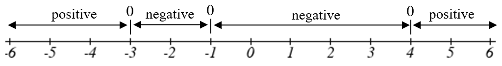
From our test values, we can determine this function is positive when \(x<-3\) or \(x>4\), or in interval notation, \((-\infty ,-3) \cup (4,\infty)\).

We could have also determined on which intervals the function was positive by sketching a graph of the function.  We illustrate that technique in the next example

Example \(\PageIndex{8}\)

Find the domain of the function \(v(t) = \sqrt {6 - 5t - t^2}\).

Solution

A square root is only defined when the quantity we are taking the square root of, the quantity inside the square root, is zero or greater.  Thus, the domain of this function will be when \(6 - 5t - t^2 \geq 0\).

Again we start by solving the equality \(6 - 5t - t^2 = 0\).  While we could use the quadratic formula, this equation factors nicely to \((6 + t)(1 - t) = 0\), giving horizontal intercepts \(t = 1\) and \(t = -6\).  Sketching a graph of this quadratic will allow us to determine when it is positive.

From the graph we can see this function is positive for inputs between the intercepts.  So \(6 - 5t - t^2 \geq 0\) for \(-6 leq t \leq 1\), and this will be the domain of the \(v(t)\) function.

Exercise \(\PageIndex{2}\)

Given the function \(g(x) = x^3 - x^2 - 6x\) use the methods that we have learned so far to find the vertical & horizontal intercepts, determine where the function is negative and positive, describe the long run behavior and sketch the graph without technology.

Answer

Vertical intercept \((0, 0)\), Horizontal intercepts \((-2, 0), (0, 0), (3, 0).\)

The function is negative on \((-\infty, -2)\) and \((0, 3)\).

The function is positive on \((-2, 0)\) and \((3,\infty)\).

The leading term is \(x^3\) so as \(x \to  - \infty, g(x) \to  -\infty\) and as \(x \to \infty, g(x) \to \infty\).

Estimating Extrema

With quadratics, we were able to algebraically find the maximum or minimum value of the function by finding the vertex.  For general polynomials, finding these turning points is not possible without more advanced techniques from calculus.  Even then, finding where extrema occur can still be algebraically challenging.  For now, we will estimate the locations of turning points using technology to generate a graph.

Example \(\PageIndex{9}\)

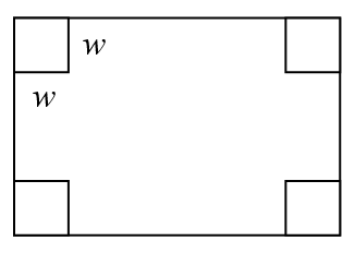An open-top box is to be constructed by cutting out squares from each corner of a 14cm by 20cm sheet of plastic then folding up the sides.  Find the size of squares that should be cut out to maximize the volume enclosed by the box.

Solution

An open-top box is to be constructed by cutting out squares from each corner of a 14cm by 20cm sheet of plastic then folding up the sides.  Find the size of squares that should be cut out to maximize the volume enclosed by the box.

We will start this problem by drawing a picture, labeling the width of the cut-out squares with a variable, \(w\).     

Notice that after a square is cut out from each end, it leaves a \((14-2w)\) cm by \((20-2w)\) cm rectangle for the base of the box, and the box will be w cm tall.  This gives the volume:

\[V(w) = (14 - 2w)(20 - 2w)w = 280w - 68{w^2} + 4w^3\nonumber\]

Using technology to sketch a graph allows us to estimate the maximum value for the volume, restricted to reasonable values for \(w\): values from 0 to 7.

 

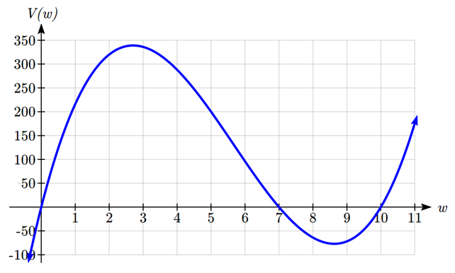
From this graph, we can estimate the maximum value is around 340, and occurs when the squares are about 2.75cm square.  To improve this estimate, we could use advanced features of our technology, if available, or simply change our window to zoom in on our graph.

 

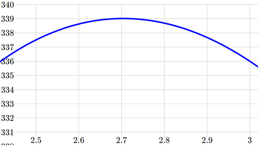
From this zoomed-in view, we can refine our estimate for the max volume to about 339, when the squares are 2.7cm square.

Exercise \(\PageIndex{3}\)

Use technology to find the maximum and minimum values on the interval \([-1, 4]\) of the function \(f(x) =  - 0.2(x - 2)^3(x + 1)^2(x - 4)\).

Answer

The minimum occurs at approximately the point \((0, -6.5)\), and the maximum occurs at approximately the point \((3.5, 7)\).

Important Topics of this Section

Vocabulary:  Polynomials, coefficients, leading coefficient, term

Degree of a polynomial

Long Run Behavior

Short Run Behavior

         Intercepts (Horizontal & Vertical)

Methods to find Horizontal intercepts

         Factoring Methods

         Factored Forms

         Technology

Graphical Behavior at intercepts

Single, Double and Triple zeros (or multiplicity 1, 2, and 3 behaviors)

Solving polynomial inequalities using test values & graphing techniques

Estimating extrema

Contributors and Attributions

• Jay Abramson (Arizona State University) with contributing authors. Textbook content produced by OpenStax College is licensed under a Creative Commons Attribution License 4.0 license. Download for free at https://openstax.org/details/books/precalculus.