4.3: Rational Functions

Last updated
Save as PDF

Page ID: 67119

$ \newcommand{\vecs}[1]{\overset { \scriptstyle \rightharpoonup} {\mathbf{#1}} } $ $ \newcommand{\vecd}[1]{\overset{-\!-\!\rightharpoonup}{\vphantom{a}\smash {#1}}} $$\newcommand{\id}{\mathrm{id}}$ $ \newcommand{\Span}{\mathrm{span}}$ $ \newcommand{\kernel}{\mathrm{null}\,}$ $ \newcommand{\range}{\mathrm{range}\,}$ $ \newcommand{\RealPart}{\mathrm{Re}}$ $ \newcommand{\ImaginaryPart}{\mathrm{Im}}$ $ \newcommand{\Argument}{\mathrm{Arg}}$ $ \newcommand{\norm}[1]{\| #1 \|}$ $ \newcommand{\inner}[2]{\langle #1, #2 \rangle}$ $ \newcommand{\Span}{\mathrm{span}}$ $\newcommand{\id}{\mathrm{id}}$ $ \newcommand{\Span}{\mathrm{span}}$ $ \newcommand{\kernel}{\mathrm{null}\,}$ $ \newcommand{\range}{\mathrm{range}\,}$ $ \newcommand{\RealPart}{\mathrm{Re}}$ $ \newcommand{\ImaginaryPart}{\mathrm{Im}}$ $ \newcommand{\Argument}{\mathrm{Arg}}$ $ \newcommand{\norm}[1]{\| #1 \|}$ $ \newcommand{\inner}[2]{\langle #1, #2 \rangle}$ $ \newcommand{\Span}{\mathrm{span}}$$\newcommand{\AA}{\unicode[.8,0]{x212B}}$

We will begin this section by looking at another economic concept. In addition to total cost and marginal cost, another metric of costs is average cost.

Definition: Average Cost

The average cost of producing $q$ items with a total cost of $C(q)$ is

\[AC(q) = \frac{C(q)}{q}\nonumber\]

Example $\PageIndex{1}$

Suppose that manufacturing an item has fixed costs of $4000 and per-item (marginal) costs of $20 per item. Find the average cost per item when 250 items are produced.

Solution

The total cost function is $C(q) = 4000 + 20q$.

Then average cost is $AC(q) = \frac{4000 + 20q}{q}$.

When 250 items are produced, the average cost per item will be

\[AC(250) = \frac{4000 + 20(250)}{250} = \$ 36 \nonumber\]

The average cost per item is $36.

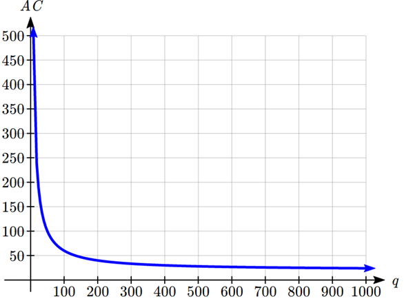
$clipboard_e6c147ab2bbf70f0bd8ef58fd83062ffb.png$

Notice that the average cost per item distributes the fixed costs across all the items. If we were to graph the average cost, notice that average costs decrease as production increases, eventually levelling off towards the per-item cost of $20.

The average cost functions is one example of a rational function.

Definition: Rational Function

A rational function is a function that can be written as the ratio of two polynomials, $P(x)$ and $Q(x)$.

\[f(x) = \frac{P(x)}{Q(x)} = \frac{a_0 + a_1x + a_2x^2 + \cdots + a_px^p}{b_0 + b_1x + b_2 x^2 + \cdots + b_q x^q}\]

To get a feel for these functions, we will look at a graph.

Example $\PageIndex{2}$

Graph $f(x) = \frac{2x + 4}{x - 3}$

Solution

Notice that the graph is undefined at x = 3, since that would cause us to divide by 0. We can create a table of values to get a sense for the function.

$x$	$f(x)$
-5	.75
-3	.333
-2	0
0	-1.333
2	-8
2.9	-98
2.99	-998
3	undefined
3.1	102
4	12
5	7

Notice that as $x$ gets close to 3 from the left, the function values are getting larger and larger in the negative direction. When $x$ is close to 3 from the right, the function values are getting large and positive. We call $x = 3$ a vertical asymptote of the function.

When $x = -2$, the function value is 0, giving a horizontal intercept. Notice that when $x=-2$ the numerator of the rational function is zero.

To get a better sense of the long run behavior, we can evaluate the function at additional, larger inputs:

$x$	$f(x)$
-1000	1.99
-100	1.90
-10	1.23
10	3.43
100	2.10
1000	2.01

Notice that as x gets large on both ends, the function approaches 2 but never actually reaches 2, it just “levels off” as the inputs become large. This behavior creates a horizontal asymptote. In this case the graph is approaching the horizontal line $f(x) = 2$as the input becomes very large in the negative and positive directions.

Sketching a graph of this function:

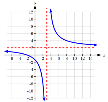
$clipboard_e01b7e9f129e8926b3d10d363aaa3a071.png$

The graphs of rational functions are sometimes sketched with the horizontal and vertical asymptotes drawn as dashed lines. It’s important to realize these are not part of the graph of the function itself.

Definition: Vertical and Horizontal Asymptotes

A vertical asymptote of a graph is a vertical line $x=1$ where the graph tends towards positive or negative infinity as the inputs approach $a$.

A horizontal asymptote of a graph is a horizontal line $y = b$ where the graph approaches the line as the inputs get large.

In the first example looking at average cost, the function had a vertical asymptote at $q=0$, and a horizontal asymptote at $AC=20$.

Finding Asymptotes and Intercepts

Given a rational function, as part of investigating the short run behavior we are interested in finding any vertical and horizontal asymptotes, as well as finding any vertical or horizontal intercepts, as we have done in the past.

To find vertical asymptotes, we notice that the vertical asymptotes in our examples occur when the denominator of the function is undefined. With one exception, a vertical asymptote will occur whenever the denominator is undefined.

Example $\PageIndex{3}$

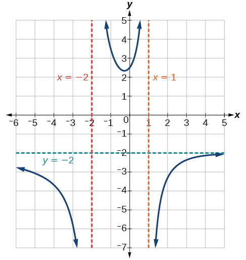
Find the vertical asymptotes of the graph of $k(x)=\frac{5+2x^2}{2−x−x^2}$.

Solution

To find the vertical asymptotes, we determine where this function will be undefined by setting the denominator equal to zero:

\[\begin{align*} 2-x-x^2&=0\\ (2+x)(1−x)&=0 \\ x& =−2,1 \end{align*}\]

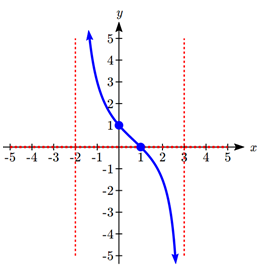
This indicates two vertical asymptotes, which a look at a graph confirms.

$Graph of k(x)=(5+2x)^2/(2-x-x^2) with its vertical asymptotes at x=-2 and x=1 and its horizontal asymptote at y=-2.$

Figure $\PageIndex{10}$.

The exception to this rule can occur when both the numerator and denominator of a rational function are zero at the same input.

Example $\PageIndex{4}$

Find the vertical asymptotes and removable discontinuities of the graph of $k(x)=\frac{x−2}{x^2−4}$.

Solution

To find the vertical asymptotes, we determine where this function will be undefined by setting the denominator equal to zero:

\[\begin{align*} x^2 - 4 = 0 \\ x^2 = 4 \\ x = - 2, 2 \end{align*} \]

However, the numerator of this function is also equal to zero when $x = 2$. Because of this, the function will still be undefined at 2, since $\frac{0}{0}$ is undefined, but the graph will not have a vertical asymptote at $x = 2$.

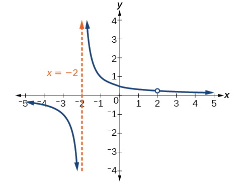
Graph of k(x)=(x-2)/(x-2)(x+2) with its vertical asymptote at x=-2 and a removable discontinuity at x=2. — Figure $\PageIndex{12}$.

The graph of this function will have the vertical asymptote at $x = -2$, but at $x = 2$ the graph will have a hole: a single point where the graph is not defined, indicated by an open circle.

Definition: Vertical Asymptotes and Holes of Rational Functions

The vertical asymptotes of a rational function will occur where the denominator of the function is equal to zero and the numerator is not zero.

A hole might occur in the graph of a rational function if an input causes both numerator and denominator to be zero. In this case, factor the numerator and denominator and simplify; if the simplified expression still has a zero in the denominator at the original input the original function has a vertical asymptote at the input, otherwise it has a hole.

To find horizontal asymptotes, we are interested in the behavior of the function as the input grows large, so we consider long run behavior of the numerator and denominator separately. Recall that a polynomial’s long run behavior will mirror that of the leading term. Likewise, a rational function’s long run behavior will mirror that of the ratio of the leading terms of the numerator and denominator functions.

There are three distinct outcomes when checking for horizontal asymptotes:

Case 1: If the degree of the denominator > degree of the numerator, there is a horizontal asymptote at $y=0$.

Example: $f(x)=\dfrac{4x+2}{x^2+4x−5}$

In this case, the end behavior is $f(x)≈\frac{4x}{x^2}=\frac{4}{x}$. This tells us that, as the inputs increase or decrease without bound, this function will behave similarly to the function $g(x)=\frac{4}{x}$, and the outputs will approach zero, resulting in a horizontal asymptote at $y=0$.

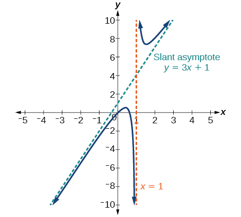
Graph of f(x)=(4x+2)/(x^2+4x-5) with its vertical asymptotes at x=-5 and x=1 and its horizontal asymptote at y=0. — Figure $\PageIndex{13}$: Horizontal asymptote $y=0$ when $f(x)=\dfrac{p(x)}{q(x)}$,$q(x)≠0$where degree of $p$ < degree of $q$.

Case 2: If the degree of the denominator < degree of the numerator by one, we get a slant asymptote.

Example: $f(x)=\dfrac{3x^2−2x+1}{x−1}$

In this case, the end behavior is $f(x)≈\frac{3x^2}{x}=3x$. This tells us that as the inputs grow large, this function will behave similarly to the function $g(x)=3x$. As the inputs grow large, the outputs will grow and not level off, so this graph has no horizontal asymptote.

Ultimately, if the numerator is larger than the denominator, the long run behavior of the graph will mimic the behavior of the reduced long run behavior fraction. As another example if we had the function $f(x) = \frac{3x^5 - x^2}{x + 3}$ with long run behavior $f(x) \approx \frac{3x^5}{x} = 3{x^4}$, the long run behavior of the graph would look similar to that of an even polynomial.

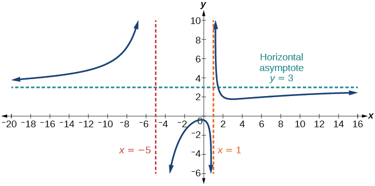
Graph of f(x)=(3x^2-2x+1)/(x-1) with its vertical asymptote at x=1 and a slant asymptote aty=3x+1. — Figure $\PageIndex{14}$: Slant asymptote when $f(x)=\frac{p(x)}{q(x)}$, $q(x)≠0$ where degree of $p$ >degree of $q$ by 1.

Case 3: If the degree of the denominator = degree of the numerator, there is a horizontal asymptote at $y=\dfrac{a_n}{b_n}$, where $a_n$ and $b_n$ are respectively the leading coefficients of $p(x)$ and $q(x)$ for $f(x)=\dfrac{p(x)}{q(x)}$, $q(x)≠0$.

Example: $f(x)=\dfrac{3x^2+2}{x^2+4x−5}$

In this case, the end behavior is $f(x)≈\dfrac{3x^2}{x^2}=3$. This tells us that as the inputs grow large, this function will behave like the function $g(x)=3$, which is a horizontal line. As $x\rightarrow \pm \infty$, $f(x)\rightarrow 3$, resulting in a horizontal asymptote at $y=3$.

Graph of f(x)=(3x^2+2)/(x^2+4x-5) with its vertical asymptotes at x=-5 and x=1 and its horizontal asymptote at y=3. — Figure $\PageIndex{15}$: Horizontal asymptote when $f(x)=\frac{p(x)}{q(x)}$, $q(x)≠0$ where degree of $p$ =degree of $q$.

HORIZONTAL ASYMPTOTES OF RATIONAL FUNCTIONS

The horizontal asymptote of a rational function can be determined by looking at the degrees of the numerator and denominator.

Degree of numerator $<$ degree of denominator: horizontal asymptote at $y=0$.
Degree of numerator $>$ degree of denominator by one: no horizontal asymptote; slant asymptote.
Degree of numerator $=$ degree of denominator: horizontal asymptote at ratio of leading coefficients.

Example $\PageIndex{5}$

Find the horizontal and vertical asymptotes of the function

\[f(x) = \frac{(x - 2)(x + 3)}{(x - 1)(x + 2)(x - 5)}\nonumber\]

Solution

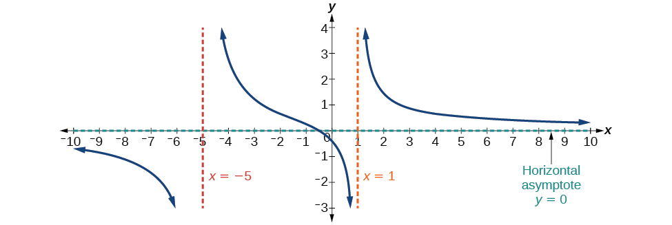
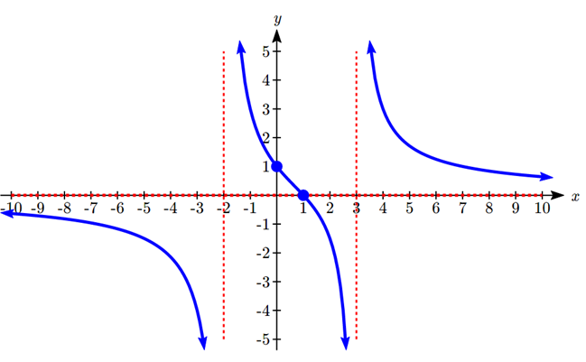
First, note this function has no inputs that make both the numerator and denominator zero, so there are no potential holes. The function will have vertical asymptotes when the denominator is zero, causing the function to be undefined. The denominator will be zero at $x=1,-2$ and $5$, indicating vertical asymptotes at these values.

The numerator has degree 2, while the denominator has degree 3. Since the degree of the denominator is greater than the degree of the numerator, the denominator will grow faster than the numerator, causing the outputs to tend towards zero as the inputs get large, and so as $x \to \pm \infty, f(x) \to 0$. This function will have a horizontal asymptote at $y = 0$.

Exercise $\PageIndex{1}$

Find the vertical and horizontal asymptotes of the function

\[f(x) = \frac{(2x - 1)(2x + 1)}{(x - 2)(x + 3)}\nonumber\]

Answer: Vertical asymptotes at $x=2$ and $x=-3$; horizontal asymptote at $y = 4$.

Example $\PageIndex{6}$

Nadi Products, an Ebay retailer that resells items purchased from Fiji, has started selling a new-to-market product. Nadi is currently selling 2,000 units a month, which has been growing by 100 units a month. The total market for the product is currently 10,000 units, but is growing by 1000 units a month.

a) Determine Nadi’s current market share

b) Find the horizontal asymptote and interpret it in context of the scenario.

Solution

Notice that the sales per month are increasing linearly. Let $t$ be the number of months, then Nadi’s sales per month are $N = 2000 + 100t$, and the total market is $M = 10000 + 1000t$.

Nadi’s market share, $MS$, the fraction of the total market that Nadi holds:

\[MS(t) = \frac{2000 + 100t}{10000 + 1000t}\nonumber\]

a) Nadi’s current market share is:

\[MS(0) = \frac{2000 + 100(0)}{10000 + 1000(0)} = \frac{2000}{10000} = 0.20 = 20\% \nonumber\]

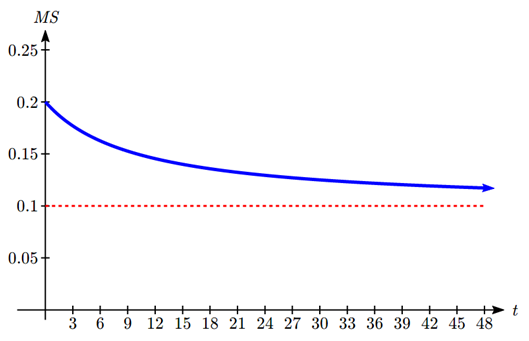
b) Both the numerator and denominator are linear (degree 1), so since the degrees are equal, there will be a horizontal asymptote at the ratio of the leading coefficients. In the numerator, the leading term is 100t, with coefficient 100. In the denominator, the leading term is 1000t, with coefficient 1000. The horizontal asymptote will be at the ratio of these values, at $y = \frac{100}{1000} = 0.10$.

This tells us that as the input gets large, the output values will approach 0.10. In context, this means that as more time goes by, Nadi’s market share will approach 10%.

$clipboard_e681e7d7b4721111822da8a454ebdebc0.png$

Intercepts

As with all functions, a rational function will have a vertical intercept when the input is zero, if the function is defined at zero. It is possible for a rational function to not have a vertical intercept if the function is undefined at zero.

Likewise, a rational function will have horizontal intercepts at the inputs that cause the output to be zero (unless that input corresponds to a hole). It is possible there are no horizontal intercepts. Since a fraction is only equal to zero when the numerator is zero, horizontal intercepts will occur when the numerator of the rational function is equal to zero.

Example $\PageIndex{7}$

Find the horizontal and vertical asymptotes of the function

\[f(x)=\dfrac{(x−2)(x+3)}{(x−1)(x+2)(x−5)}\]

Solution

We can find the vertical intercept by evaluating the function at zero

\[f(0) = \frac{(0 - 2)(0 + 3)}{(0 - 1)(0 + 2)(0 - 5)} = \frac{-6}{10} = - \frac{3}{5} \nonumber \]

The horizontal intercepts will occur when the function is equal to zero:

\[\begin{align*} 0 &= \frac{(x - 2)(x + 3)}{(x - 1)(x + 2)(x - 5)}& \text{This is zero when the numerator is zero} \\0 &= (x - 2)(x + 3) & \\ x &= 2, - 3 & \end{align*}\]

Example $\PageIndex{8}$

Sketch a graph of $f(x) = \frac{6(x - 1)}{(x + 2)(x - 3)}$.

Solution

We can start our sketch by finding intercepts and asymptotes. Evaluating the function at zero gives the vertical intercept:

\[f(0) = \frac{6(0 - 1)}{(0 + 2)(0 - 3)} = \frac{- 6}{- 6} = 1\nonumber\]

Looking at when the numerator of the function is zero, we can determine the graph will have a horizontal intercept at $x=1$.

Looking at when the denominator of the function is zero, we can determine the graph will have vertical asymptotes at $x = -2$ and $x = 3$.

Finally, the degree of denominator is larger than the degree of the numerator, telling us this graph has a horizontal asymptote at $y = 0$.

To sketch the graph, we might start by plotting the intercepts and drawing the asymptotes as dashed lines.

$clipboard_efa295012307a917b3f62d30c574b6d51.png$

We can now try to sketch a smooth curve passing through both intercepts. As the graph approaches $x=3$, the graph must approach negative infinity. As we sketch from $x=0$ towards $x=-2$, we’d expect the graph to approach positive infinity.

To finish the curve, we need to fill in the portions to the right of $x=3$ and to the left of $x=-2$. If we evaluate the function to the right of $x=3$ we’d see the output is positive, indicating the graph will decrease from positive infinity then level off towards the horizontal asymptote of $y=0$. To the left of $x=-2$ the graph will also level off at the horizontal asymptote, and will approach negative infinity to the left of the asymptote.

$clipboard_e4c6349e5921519a15e360b9dbb838c1d.png$

Exercise $\PageIndex{2}$

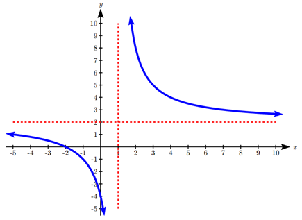
Given the function $f(x) = \frac{2(x + 2)}{x - 1}$, find the intercepts and asymptotes and sketch the function.

Answer

Horizontal asymptote at $y = 2$.

Vertical asymptote is at $x = 1$.

Vertical intercept at $(0, 4)$.

Horizontal intercept $(2, 0)$.

$clipboard_e98b71e75d81235a3ead5481283b49bf7.png$

Important Topics of this Section

Horizontal Asymptotes

Vertical Asymptotes

Rational Functions

Finding intercepts, asymptotes, and holes

Given equation sketch the graph

Contributor

Jay Abramson (Arizona State University) with contributing authors. Textbook content produced by OpenStax College is licensed under a Creative Commons Attribution License 4.0 license. Download for free at https://openstax.org/details/books/precalculus.

\(x\)	\(f(x)\)
-5	.75
-3	.333
-2	0
0	-1.333
2	-8
2.9	-98
2.99	-998
3	undefined
3.1	102
4	12
5	7