2.2: Graphing on the Cartesian Coordinate Plane

Last updated
Save as PDF

Page ID: 108415

$ \newcommand{\vecs}[1]{\overset { \scriptstyle \rightharpoonup} {\mathbf{#1}} } $ $ \newcommand{\vecd}[1]{\overset{-\!-\!\rightharpoonup}{\vphantom{a}\smash {#1}}} $$\newcommand{\id}{\mathrm{id}}$ $ \newcommand{\Span}{\mathrm{span}}$ $ \newcommand{\kernel}{\mathrm{null}\,}$ $ \newcommand{\range}{\mathrm{range}\,}$ $ \newcommand{\RealPart}{\mathrm{Re}}$ $ \newcommand{\ImaginaryPart}{\mathrm{Im}}$ $ \newcommand{\Argument}{\mathrm{Arg}}$ $ \newcommand{\norm}[1]{\| #1 \|}$ $ \newcommand{\inner}[2]{\langle #1, #2 \rangle}$ $ \newcommand{\Span}{\mathrm{span}}$ $\newcommand{\id}{\mathrm{id}}$ $ \newcommand{\Span}{\mathrm{span}}$ $ \newcommand{\kernel}{\mathrm{null}\,}$ $ \newcommand{\range}{\mathrm{range}\,}$ $ \newcommand{\RealPart}{\mathrm{Re}}$ $ \newcommand{\ImaginaryPart}{\mathrm{Im}}$ $ \newcommand{\Argument}{\mathrm{Arg}}$ $ \newcommand{\norm}[1]{\| #1 \|}$ $ \newcommand{\inner}[2]{\langle #1, #2 \rangle}$ $ \newcommand{\Span}{\mathrm{span}}$$\newcommand{\AA}{\unicode[.8,0]{x212B}}$

Learning Objectives

By the end of this section you will be able to...

Plot ordered pairs on the Cartesian plane
Compute the distance between two points on the Cartesian coordinate plane
Compute the midpoint between two points on the Cartesian coordinate plane
Graph relations and functions defined with ordered pairs
Graph functions defined with an equation using a table to create ordered pairs

Warm Up $\PageIndex{1}$

Identify the $x$ and $y$ values in each ordered pair below.

$(1, 3)$
$(4, -2)$
$(-25, -72)$

Answer

For $(1, 3)$, the $x$ value is 1 and the $y$ value is 3.
For $(4, -2)$, the $x$ value is 4 and the $y$ value is -2.
For $(-25, -72$, the $x$ value is -25 and the $y$ value is -72.

The Cartesian Coordinate Plane

In the previous section, we talked about how we can use ordered pairs to form the building blocks of relations and functions. We introduced a few ways to understand these types of relationships between numbers, including lists of ordered pairs, mapping diagrams, tables, and in the case of functions, writing an equation. In this section, we look at a new way to understand the relationships between numbers by visualizing the ordered pairs on a graph.

To create a graph, we start with what is called the Cartesian Coordinate Plane. The Cartesian coordinate plane, shown below, uses a grid system to plot ordered pairs using two number lines at the same time called the $x$-axis and $y$-axis. The place these axes intersect is called the origin. For an ordered pair $(x, y)$, the $x$-axis displays the first coordinate by moving along the horizontal direction and the $y$-axis displays the second coordinate by moving along the vertical direction. For positive numbers, we move either right (for the $x$ component) or up (for the $y$ component). For negative numbers, we move either left (for the $x$ component) or down (for the $y$ component). The origin is located at the point (0, 0); this is where we always start before moving along the $x$ or $y$ axis to plot a point.

$Fig: Cartesian coordinate plane$

Caution

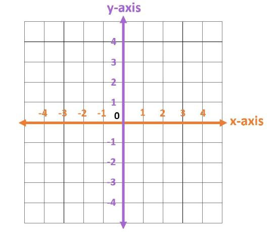
When plotting, the first component gives horizontal information, and the second component gives vertical information. The order of the ordered pair is very important; they are not interchangeable!

Let's look at some examples on how to plot points.

Example $\PageIndex{1}$

Plot the following on a Cartesian coordinate plane:

(1, 2)
(-3, 4)
(2, -1)

Solution

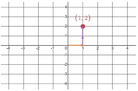
To plot the point (1, 2), starting at the origin (0, 0), we first go right 1 unit along the $x$ axis, then up 2 units along the $y$ axis.

$pt_1_2_plot.JPG$

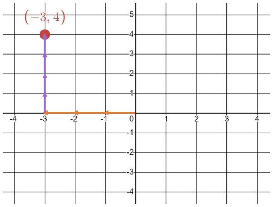
To plot the point (-3, 4), starting at the origin (0, 0), we first go left 3 units along the $x$ axis, then up 4 units along the $y$ axis.

$pt_neg3_4_plot.JPG$

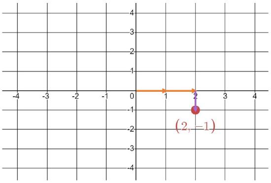
To plot the point (2, -1), starting at the origin (0, 0), we first go right 2 units along the $x$ axis, then down 1 unit along the $y$ axis.

$pt_2_neg1_plot.JPG$

Exercise $\PageIndex{2}$

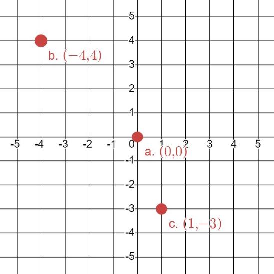
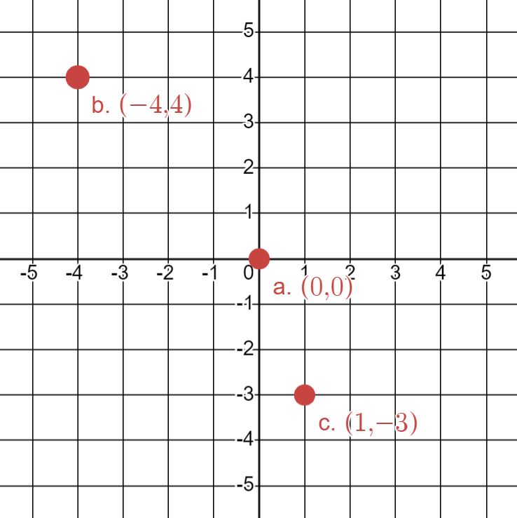
Plot the following on a Cartesian coordinate plane.

(0, 0)
(-4, 4)
(1, -3)

Answer: $plot_pts_ex2.JPG$

It is also useful to be able to look at a point on a graph and be able to identify the corresponding ordered pair.

Example $\PageIndex{3}$

Identify the ordered pairs for the points shown on the graph below.

$id_pts_ex1.JPG$

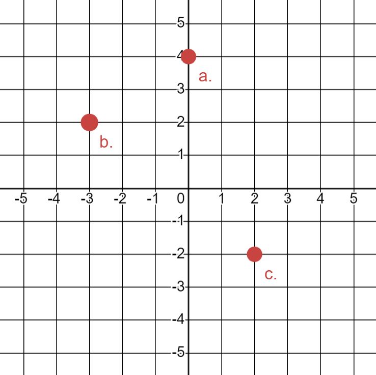
Solution

The point is directly over the origin, so we haven't moved left or right. Therefore, the $x$ value is 0. It's 4 units up, so the $y$ value is 4. Therefore, the ordered pair is (0, 4).
Starting at the origin, this point is 3 units to the left, so the $x$ value is -3. From there, it's 2 units up, so the $y$ value is 2. Therefore, the ordered pair is (-3, 2).
Starting at the origin, the point is 2 units to the right, so the $x$ value is 2. From there, it's 2 units down, so the $y$ value is -2. Therefore, the ordered pair is (2, -2).

Exercise $\PageIndex{4}$

Identify the ordered pairs for the points shown on the graph below.

$id_pts_ex2.JPG$

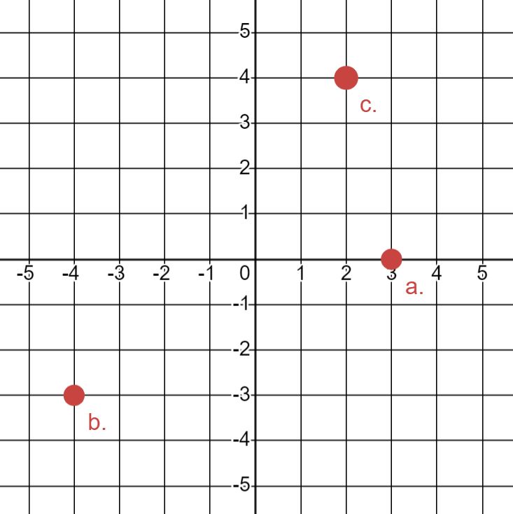
Answer

Add texts here. Do not delete this text first.

(3, 0)
(-4, -3)
(2, 4)

Computing Distance between Two Points

It is useful to be able to talk about the distance between two points plotted on a graph. Suppose we have two points $(x_1, y_1)$ and $(x_2, y_2)$. We can use a formula based on the Pythagorean theorem to determine the distance between these two points.

$distance_between_pts.JPG$

Definition:DISTANCE FORMULA

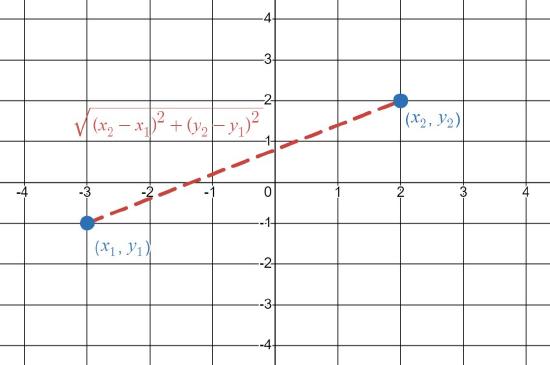
To compute the distance between two points $(x_1, y_1)$ and $(x_2, y_2)$ on a graph, we use the following formula:

$d = \sqrt{(x_2 - x_1)^2 + (y_2 - y_1)^2}.$

Let's try this out with a few examples!

Example $\PageIndex{5}$

Compute the distance between the following two points: (1, 2), (5, 5)

Solution

We have $(x_1, y_1) = (1, 2)$ and $(x_2, y_2) = (5, 5)$. Therefore the distance between these two points is

$d = \sqrt{(5 - 1)^2 + (5 - 2)^2} = \sqrt{4^2 + 3^2} = \sqrt{16 + 9} = \sqrt{25} = 5$.

Exercise $\PageIndex{6}$

Compute the distance between the following two points: (-1, 4), (5, 12)

Answer

We have $(x_1, y_1) = (-1, 4)$ and $(x_2, y_2) = (5, 12)$. Therefore the distance between these two points is

$d = \sqrt{(5 - (-1))^2 + (12 - 4)^2} = \sqrt{6^2 + 8^2} = \sqrt{36 + 64} = \sqrt{100} = 10$.

Exercise $\PageIndex{7}$

Compute the distance between the following two points: (3, 5), (15, 0)

Answer

We have $(x_1, y_1) = (3, 5)$ and $(x_2, y_2) = (15, 0)$. Therefore the distance between these two points is

$d = \sqrt{(15 - 3)^2 + (0 - 5)^2} = \sqrt{12^2 + (-5)^2} = \sqrt{144 + 25} = \sqrt{169} = 13$.

Computing the Midpoint of Two Points

We can also determine the midpoint for two points. That is, if we are given two points, it is possible to figure out a third point that is located exactly halfway between the two original points.

$midpt.JPG$

Definition: MIDPOINT FORMULA

To compute the midpoint between two points $(x_1, y_1)$ and $(x_2, y_2)$ on a graph, we use the following formula:

$\left(\frac{x_2 + x_1}{2}, \frac{y_2 + y_1}{2}\right).$

Using this formula, computing the midpoint of two points very straightforward. It's essentially finding their average $x$ value and their average $y$ value.

Example $\PageIndex{8}$

Find the midpoint for the following two points: (-1, 3), (2, 5)

Solution

We have $(x_1, y_1) = (-1, 3)$ and $(x_2, y_2) = (2, 5)$. Therefore the midpoint has coordinates

$\left(\frac{-1 + 2}{2}, \frac{3 + 5}{2}\right) = \left(\frac{1}{2}, \frac{8}{2}\right) = \left(\frac{1}{2}, 4\right)$.

Exercise $\PageIndex{9}$

Find the midpoint for the following two points: (0, 8), (-4, 10)

Answer: (-2, 9)

Exercise $\PageIndex{10}$

Find the midpoint for the following two points: (-2, -4), (0, -6)

Answer: (-1, -5)

Graphing Relations and Functions

The biggest use for graphs is that it allows us to actually visualize the relations and functions that we are working with. In order to do this, we simply graph the ordered pairs in the relation or function on the Cartesian coordinate plane.

Example $\PageIndex{11}$

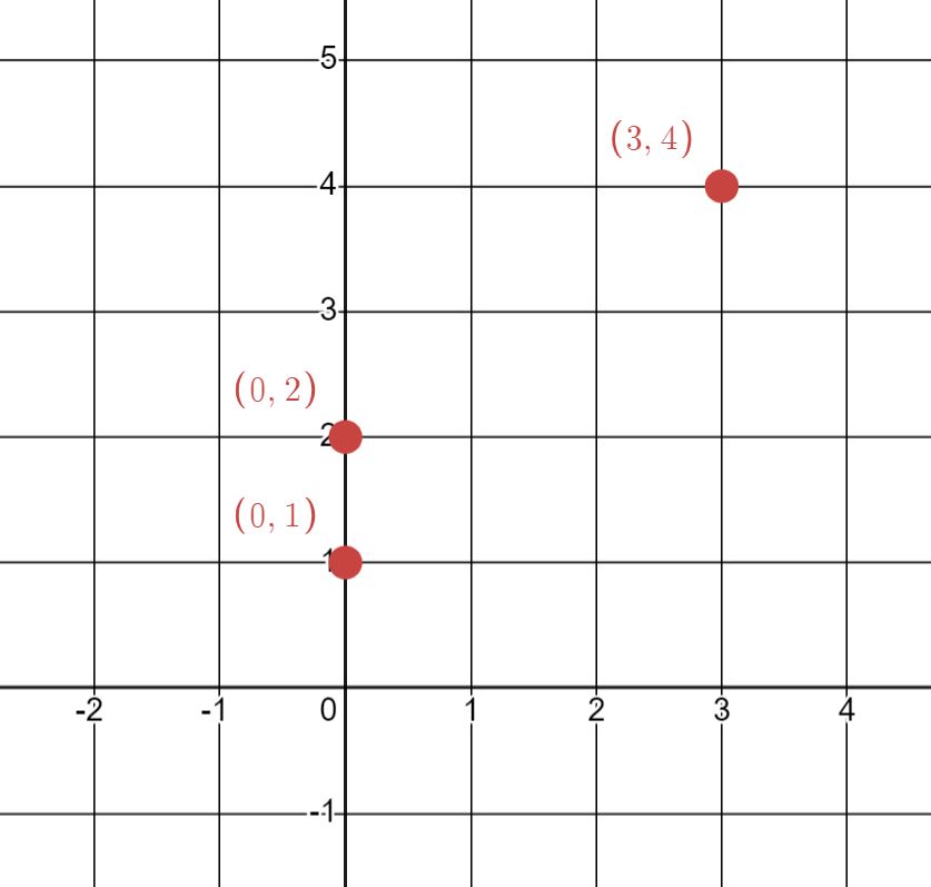
Graph the relation $R = \{(0,1),(0,2),(3,4)\}$

Solution

$graph_rel_ex1.JPG$

Exercise $\PageIndex{12}$

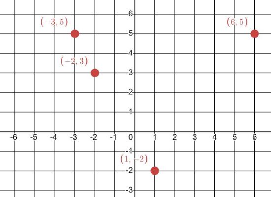
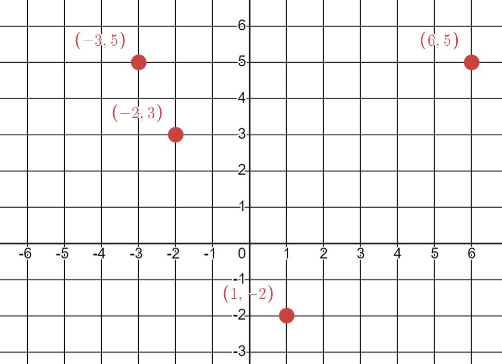
Graph the relation $R = \{(-3, 5), (-2, 3), (0, 12), (1, -2), (6, 5)\}$

Answer: $graph_rel_ex2.JPG$

Example $\PageIndex{13}$

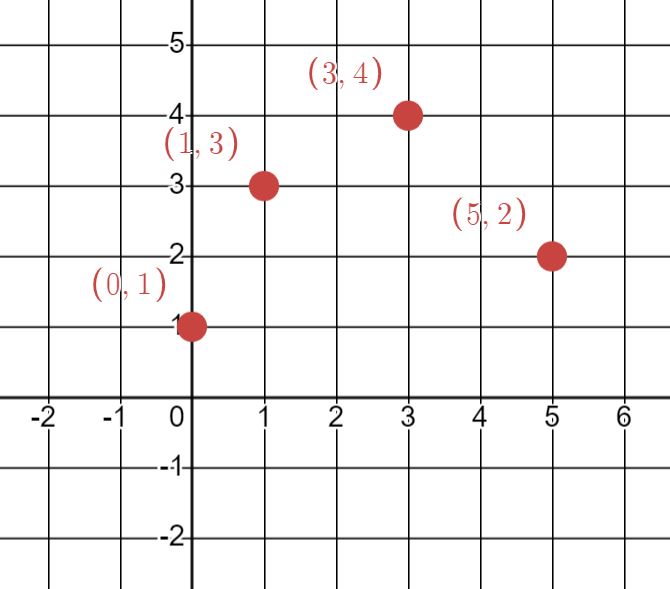
Graph the function $\{(0,1),(1,3),(3,4),(5,2)\}$

Solution

$graph_funct_ex1.JPG$

Exercise $\PageIndex{14}$

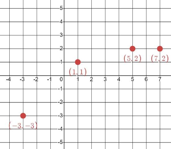
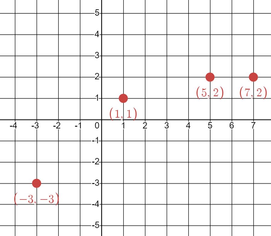
Graph the function $\{(−3,−3),(1,1),(5,2),(7,2)\}$

Answer: $graph_funct_ex2.JPG$

The process is pretty straightforward when we are given the ordered pairs to plot! But in the last section, we discussed how functions can be described by rules using equations, instead of a short list of ordered pairs. This means that in order to create ordered pairs to graph the function, we must choose our own inputs for this. For each input $x$, the resulting ordered pair becomes

$(x, f(x)).$

These ordered pairs will act as our ordered pairs $(x, y)$ that we use for plotting, where we treat $f(x)$ as the $y$ values.

We can choose a list of several convenient inputs that will help us determine the general shape of a function, collect inputs and outputs in a table, then create ordered pairs from them. These are what we will use to graph a function $f(x)$ that we determine using an equation.

Example $\PageIndex{15}$

Graph $f(x) = 2x-1$ using a table.

Solution

Step 1: Create a table to keep track of inputs, outputs, and ordered pairs.

$\begin{array} {|c|c|}\hline \text{Inputs \((x)$} & \text{Outputs $f(x)$} & \text{Ordered Pairs $(x, f(x))$} \\ \hline & & \\ \hline & & \\ \hline & & \\ \hline & & \\ \hline & & \\ \hline \end{array}\)

Step 2: Choose several inputs to use to create ordered pairs; convenient numbers such as -1, 0, 1 are good to include, and often times, 4-5 points is sufficient to get an idea of what the graph will look like. Add these inputs to the table.

In this example, we will use $x$ values -2, -1, 0, 1, 2; but you can use whatever values you wish.

$\begin{array} {|c|c|}\hline \text{Inputs \((x)$} & \text{Outputs $f(x)$} & \text{Ordered Pairs $(x, f(x))$} \\ \hline -2 & & \\ \hline -1 & & \\ \hline 0 & & \\ \hline 1 & & \\ \hline 2 & & \\ \hline \end{array}\)

Step 3: Compute the outputs $f(x)$ corresponding to each input $x$ by plugging the $x$ value into the rule for $f(x)$; add these to the table.

$\begin{array} {|c|c|}\hline \text{Inputs \((x)$} & \text{Outputs $f(x)$} & \text{Ordered Pairs $(x, f(x))$} \\ \hline -2 & 2 \cdot (-2) - 1 = -5 & \\ \hline -1 & 2 \cdot (-1) - 1 = -3 & \\ \hline 0 & 2 \cdot 0 - 1 = -1 & \\ \hline 1 & 2 \cdot 1 - 1 = 1 & \\ \hline 2 & 2 \cdot 2 - 1 = 3 & \\ \hline \end{array}\)

Step 4: Create ordered pairs from the inputs and their outputs; add to table

$\begin{array} {|c|c|}\hline \text{Inputs \((x)$} & \text{Outputs $f(x)$} & \text{Ordered Pairs $(x, f(x))$} \\ \hline -2 & 2 \cdot (-2) - 1 = -5 & (-2, -5) \\ \hline -1 & 2 \cdot (-1) - 1 = -3 & (-1, -3) \\ \hline 0 & 2 \cdot 0 - 1 = -1 & (0, -1) \\ \hline 1 & 2 \cdot 1 - 1 = 1 & (1, 1) \\ \hline 2 & 2 \cdot 2 - 1 = 3 & (2, 3) \\ \hline \end{array}\)

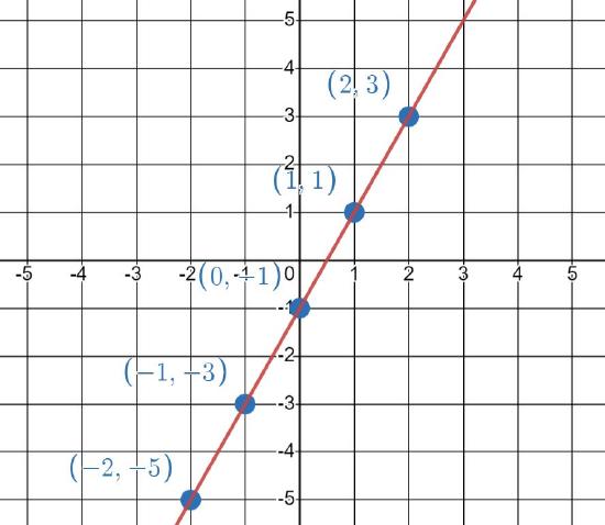
Step 5: Use the ordered pairs to plot the graph of the function. Based on the table we have created, we need to plot the pairs (-2, -5), (-1, -3), (0, 1), (1, 1), and (2, 3):

$ex_plot_funct_2x_neg1.JPG$

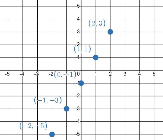
Step 6: Draw the function by connecting the dots. Recall that when a function is defined by an equation, we have a lot of inputs for $x$ to choose from. We account for this on the graph by sketching a picture of a graph suggested by the points plotted. In this case, the graph turns out to be a straight line. Be sure to continue the line beyond the last points to indicate that we could have used even more inputs!

$ex_plot_funct_2x_neg1_line.JPG$

Exercise $\PageIndex{16}$

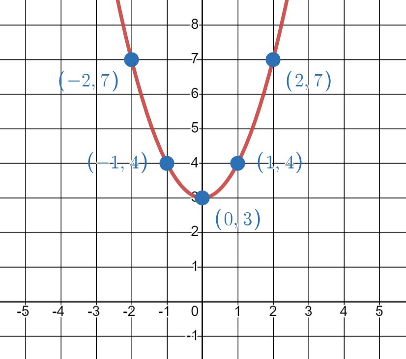
Graph the function $f(x) = x^2 + 3$ using a table.

Answer

The points used on the table may vary, but the graph should look the same.

Table	Graph
$\begin{array} {\|r\|r\|}\hline \text{Inputs \((x)$} & \text{Outputs $f(x)$} & \text{Ordered Pairs $(x, f(x))$} \\ \hline -2 & 7 & (-2, 7) \\ \hline -1 & 4 & (-1, 4) \\ \hline 0 & 3 & (0, 3) \\ \hline 1 & 4 & (1, 4) \\ \hline 2 & 7 & (2, 7) \\ \hline \end{array}\)	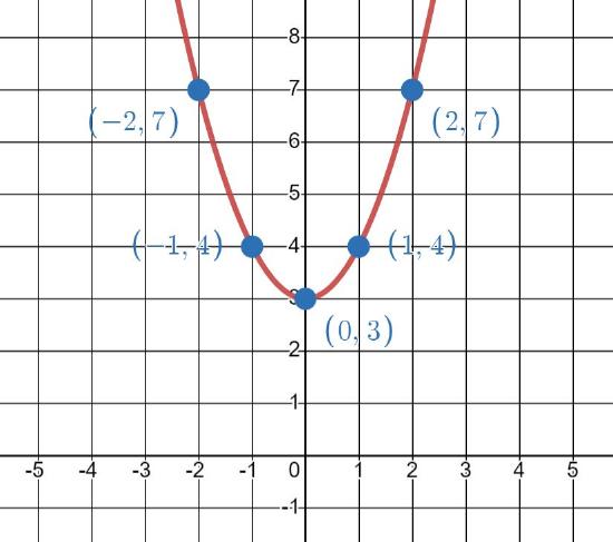$graph_funct_table_ex2.JPG$

Key Concepts

The Cartesian coordinate plane allows us to visualize ordered pairs by representing the inputs along horizontal number line called the $x$ axis and outputs along a vertical number line called the $y$ axis.
How to plot an ordered pair
1. Start at the origin (0, 0); this is where the axes intersect
2. Move the number of units in the $x$ component horizontally. If $x$ is positive, move right. If $x$ is negative, move left.
3. Move the number of units in the $y$ component vertically. If $y$ is positive, move up. If $y$ is negative, move down.
We can compute the distance between two points $(x_1, y_1)$ and $(x_2, y_x)$ by using the equation

$d = \sqrt{(x_2 - x_1)^2 + (y_2 - y_1)^2}.$

We can compute the midpoint of two points $(x_1, y_1)$ and $(x_2, y_x)$ by using the equation

$\left(\frac{x_2 + x_1}{2}, \frac{y_2 + y_1}{2}\right).$

To graph a function defined using an equation for its rule
1. Create a table to keep track of inputs, outputs, and ordered pairs.
2. Choose several inputs to use to create ordered pairs; convenient numbers such as -1, 0, 1 are good to include, and often times, 4-5 points is sufficient to get an idea of what the graph will look like. Add these inputs to the table.
3. Compute the outputs $f(x)$ corresponding to each input $x$ by plugging the $x$ value into the rule for $f(x)$; add these to the table.
4. Create ordered pairs from the inputs and their outputs; add to table
5. Use the ordered pairs to plot the graph of the function.
6. Draw the function by connecting the dots. Recall that when a function is defined by an equation, we have a lot of inputs for $x$ to choose from. We account for this on the graph by sketching a picture of a graph suggested by the points plotted. Be sure to continue the graph beyond the last points to indicate that we could have used even more inputs!