2.4: Families of Functions

Learning Objectives

• Identify families of functions based on their rule
• Identify families of functions based on their graphs
• Match functions and their graphs based on their family

Families of Functions

In the last few sections, we've studied functions and how we can represent them visually using a graph. So far, we've looked a wide variety of functions, and in some of the examples, you may have noticed that the resulting graphs looked really similar to each other. As it turns out, there are "families" of functions based on equations that result in specific shapes of graphs, where the only difference between them may be that they've been moved around or flipped over. In this section, we will identify the main families of functions and their graphs we are going to work with in this class. Of course, there are many more families of functions than we will talk about here, but these particular families will be the focus of our class!

Linear Functions

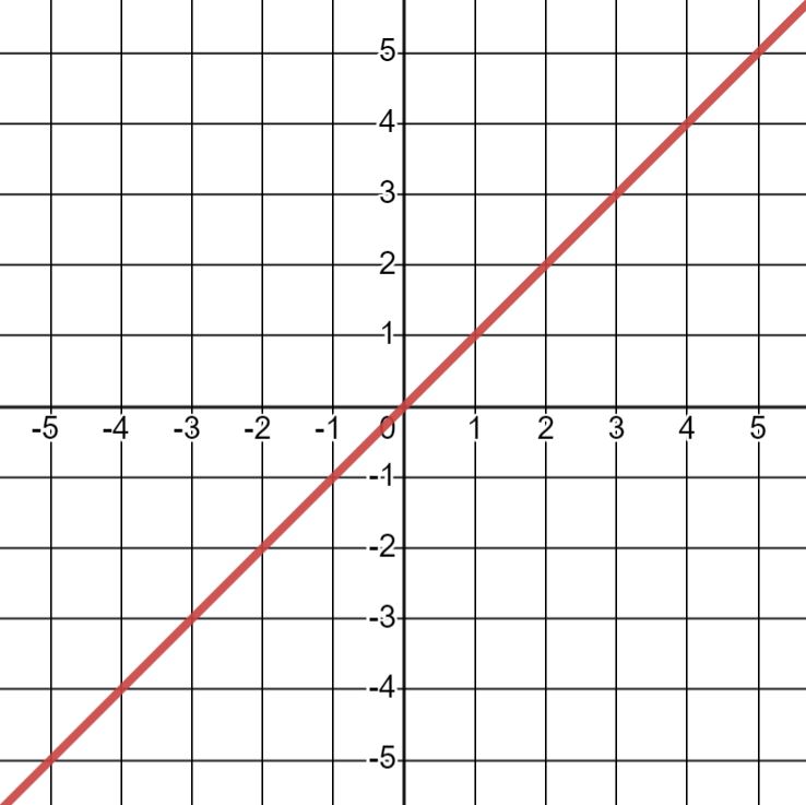
Our first family of functions is called linear functions. The "parent" function for this family is

\(f(x) = x\).

As you may have guessed, these are the type of functions whose graphs are a straight line. The graph of \(f(x) = x\) looks like

Graphs in this family may have different slants or be in a different location on the coordinate plane, but what they all have in common is their basic shape is a straight line. Their rules also all look similar, where the equation only has \(x\) which may be multiplied by a constant or have a constant added to it, but that's it. Let's plot some other examples of linear functions:

Example \(\PageIndex{1}\)

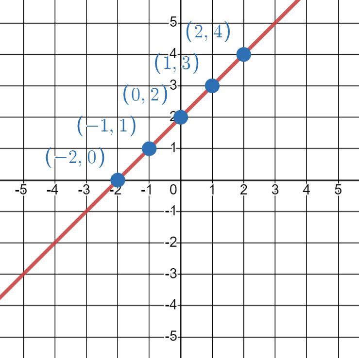
Graph the following linear function using a table: \(f(x) = x + 2\)

Solution

First, let's make a table of ordered pairs we can plot; five points should be sufficient to create the graph

\(\begin{array} {|c|c|}\hline \boldsymbol{x} & \boldsymbol{f(x)} & \boldsymbol{(x, f(x))} \\ \hline -2 & -2 + 2 = 0 & (-2, 0) \\ \hline -1 & -1 + 2 = 1 & (-1, 1) \\ \hline 0 & 0 + 2 = 2 & (0, 2) \\ \hline 1 & 1 + 2 = 3 & (1, 3) \\ \hline 2 & 2 + 2 = 4 & (2, 4) \\ \hline \end{array}\)

Now let's plot the ordered pairs on a coordinate plane.

Finally, we add the line.

Example \(\PageIndex{2}\)

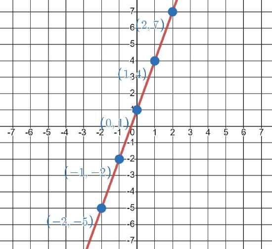
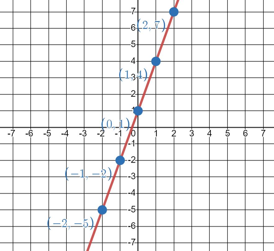
Graph the following linear function using a table: \(f(x) = 3x + 1\)

Answer

Table	Graph
\(\begin{array} {|c|c|}\hline x & f(x) & (x, f(x)) \\ \hline -2 & -5 & (-2, -5) \\ \hline -1 & -2 & (-1, -2) \\ \hline 0 & 1 & (0, 1) \\ \hline 1 & 4 & (1, 4) \\ \hline 2 & 7 & (2, 7) \\ \hline \end{array}\)

Exercise \(\PageIndex{3}\)

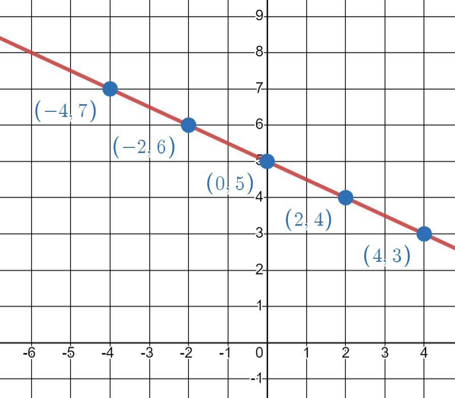
Graph the following linear function using a table: \(f(x) = -\frac{1}{2}x + 5\)

Answer

Table	Graph
\(\begin{array} {|c|c|}\hline x & f(x) & (x, f(x)) \\ \hline -4 & 7 & (-4, 7) \\ \hline -2 & 6 & (-2, 6) \\ \hline 0 & 5 & (0, 5) \\ \hline 2 & 4 & (2, 4) \\ \hline 4 & 3 & (4, 3) \\ \hline \end{array}\)

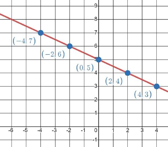
Other Linear Graphs

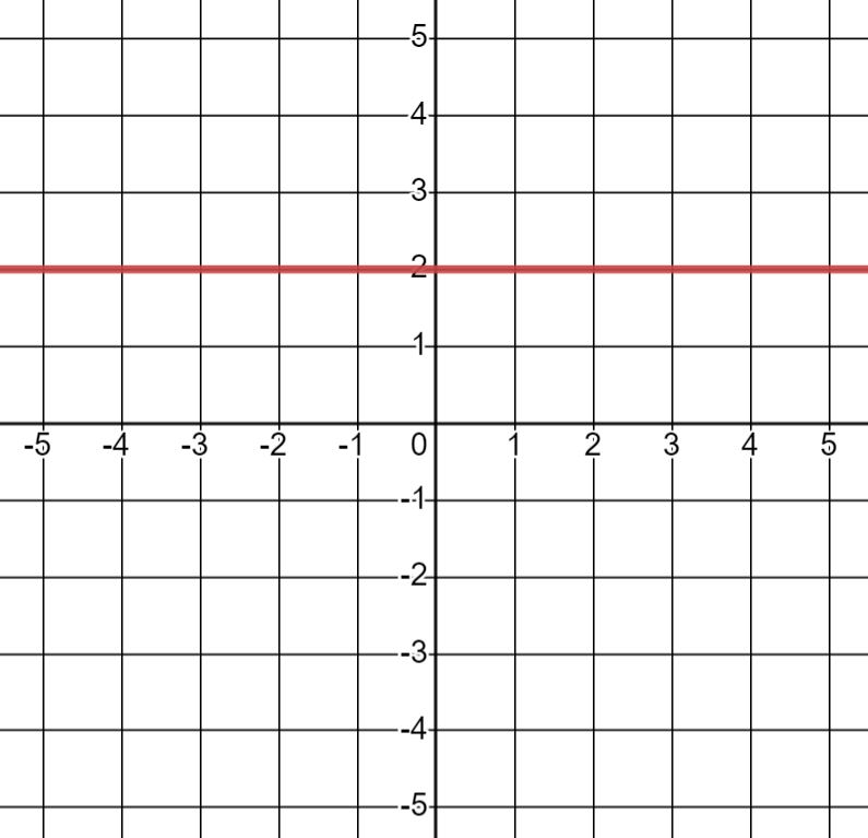
We should also mention two other types of equations that result in graphs that are straight lines. The first is the function \(f(x) = a\), where \(a\) is any number. This means that regardless of what \(x\) is, the output is always the same. The result is a horizontal line at the height of \(a\) since the \(y\) components are all equal to \(a\).

Example \(\PageIndex{4}\)

Graph the function \(f(x) = 2\).

Solution

The graph of \(f(x) = 2\) is just a horizontal line at \(y = 2\).

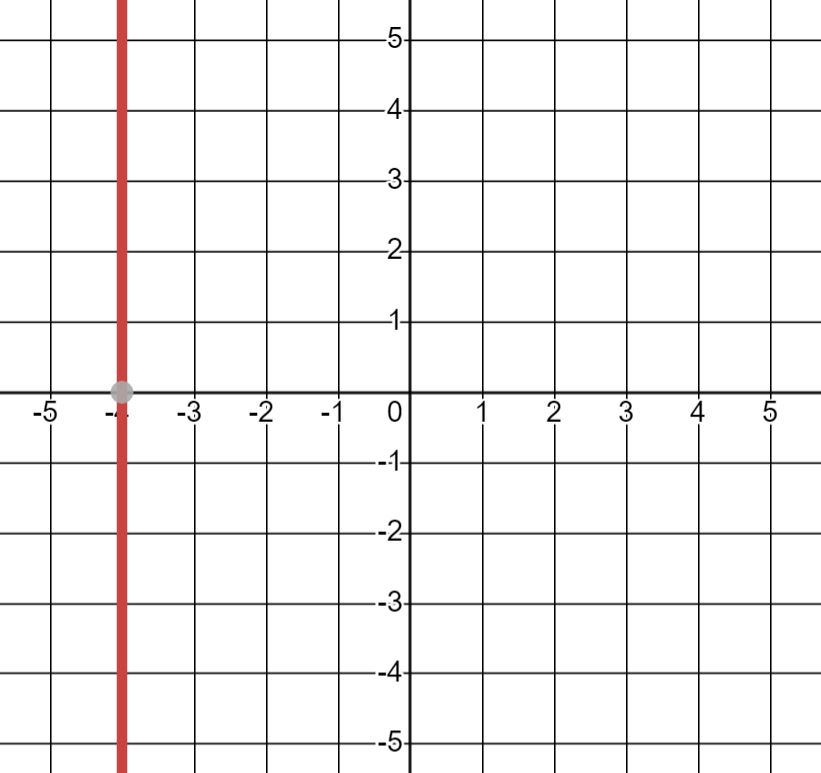
Another equation that results in a straight line is the equation \(x = a\), where we only consider a single value of \(x\) and then allow \(y\) to be anything. This results in a vertical line at \(x = a\). However, it is important to notice that a vertical line does NOT represent a function, as it would not pass the vertical line test (the one \(x\) value has infinitely many \(y\) values corresponding to it!).

Example \(\PageIndex{5}\)

Graph the line \(x = -4\)

Solution

The graph of \(x = -4\) is just a vertical line at \(x = -4\).

Absolute value

Our next family of functions is those that look like linear functions, but incorporate an absolute value. We might recall that the absolute values return the positive version of whatever is inside of it. Intuitively, if we have a positive number then we don't do anything; if we have a negative number then we make it into a positive.

One way to think of this is as being a function that has two rules, one where we do nothing and one where we multiply negative values by a negative to make it a positive.

Definition: Absolute value function

\begin{equation*}
f(x) = \lvert x \rvert = \left\{
\begin{array}{ll}
-x & \quad x \leq 0 \\
x & \quad x \geq 0
\end{array}
\right.
\end{equation*}

The "parent" function for this family of functions is

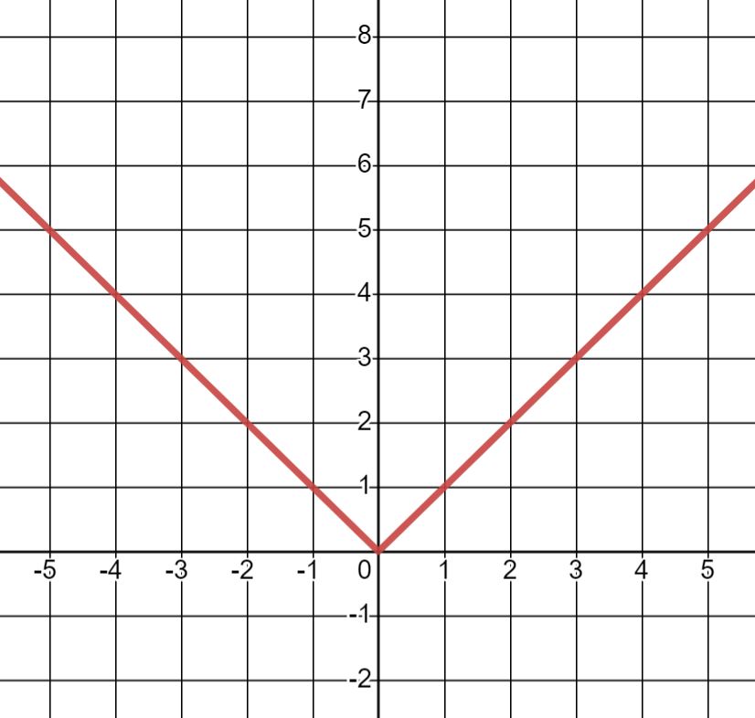
\(f(x) = |x|\).

It has a graph similar to the linear graph, except it has a "v" shape due to the absolute value changing the sign on half of the graph.

All functions in this family will have graphs with this basic shape; however, they may be moved, flipped over (depending on how the rule has been changed, the graph may not always be positive!), or stretched. Let's look at some other examples of functions in this family.

Our first example has been moved around horizontally.

Example \(\PageIndex{6}\)

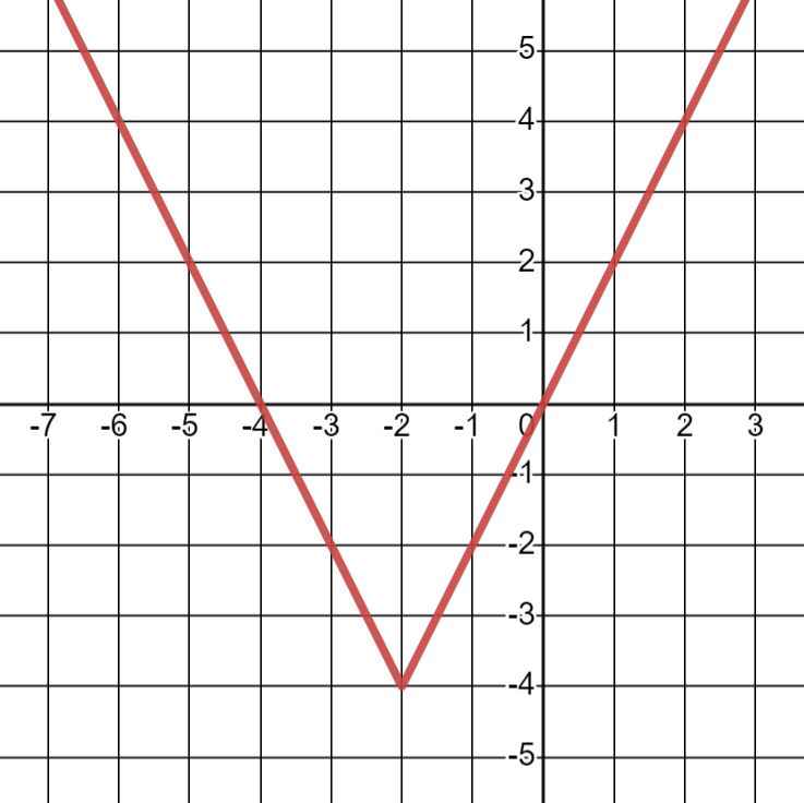
Graph the following absolute value function using a table: \(f(x)=|x-2|\)

Solution

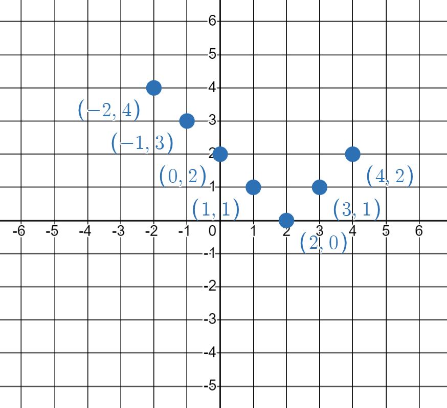
First, let's make a table to contain ordered pairs for plotting. We need to make sure include enough points to understand the shape of the graph. Since we expect the absolute value to have a "v" shape, we will use a couple more than we normally would.

\(\begin{array} {|c|c|}\hline x & f(x) & (x, f(x)) \\ \hline -2 & |-2 - 2| = |-4| = 4 & (-2, 4) \\ \hline -1 & |-1 - 2| = |-3| = 3 & (-1, 3) \\ \hline 0 & |0 - 2| = |-2| = 2 & (0, 2) \\ \hline 1 & |1 - 2| = |-1| = 1 & (1, 1) \\ \hline 2 & |2 - 2| = |0| = 0 & (2, 0) \\ \hline 3 & |3 - 2| = |1| = 1 & (3, 1) \\ \hline 4 & |4 - 2| = |2| = 2 & (4, 2) \\ \hline \end{array}\)

Let's plot the points.

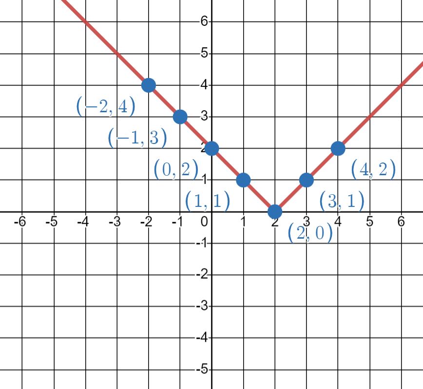
Finally, we sketch the graph. We use both the dots and the knowledge that we expect a "v" shape to do this.

Our next example has been moved vertically.

Example \(\PageIndex{7}\)

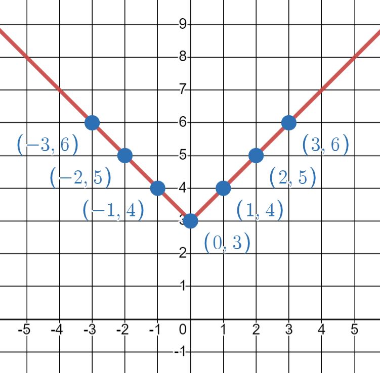
Graph the following absolute value function using a table: \(f(x)=|x|+3\)

Answer

Table	Graph
\(\begin{array} {|c|c|}\hline x & f(x) & (x, f(x)) \\ \hline -3 & |-3| + 3 = 3 + 3 = 6 & (-3, 6) \\ \hline -2 & |-2| + 3 = 2 + 3 = 5 & (-2, 5) \\ \hline -1 & |-1| + 3 = 1 + 3 = 4 & (-1, 4) \\ \hline 0 & |0| + 3 = 0 + 3 = 3 & (0, 3) \\ \hline 1 & |1| + 3 = 1 + 3 = 4 & (1, 4) \\ \hline 2 & |2| + 3 = 2 + 3 = 5 & (2, 5) \\ \hline 3 & |3| + 3 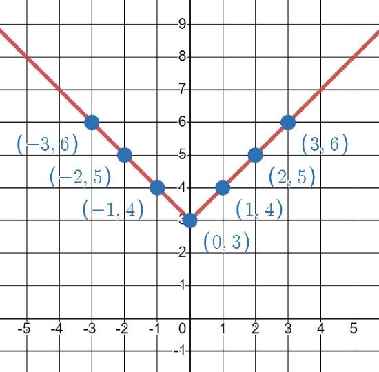= 3 + 3 = 6 & (3, 6) \\ \hline \end{array}\)

One more example! This time, our graph has been moved horizontally, vertically, and flipped over!

Example \(\PageIndex{8}\)

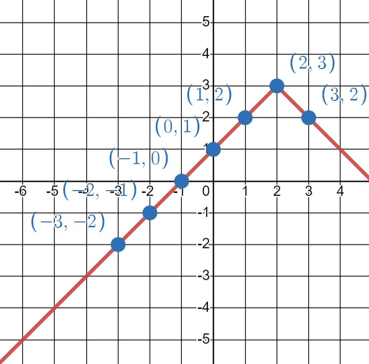
Graph the following absolute value function using a table: \(f(x)=-|x-2|+3\)

Answer

Table

Graph

\(\begin{array} {|c|c|}\hline x & f(x) & (x, f(x)) \\ \hline -3 & -|-3 - 2| + 3 = -|-5| + 3 = -(5) + 3 = -2 & (-3, -2) \\ \hline -2 & -|-2 - 2| + 3 = -|-4| + 3 = -(4) + 3 = -1 & (-2, -1) \\ \hline -1 & -|-1 - 2| + 3 = -|-3| + 3 = -(3) + 3 = 0 & (-1, 0) \\ \hline 0 & -|0 - 2| + 3 = -|-2| + 3 = -(2) + 3 = 1 & (0, 1) \\ \hline 1 & -|1 - 2| + 3 = -|-1| + 3 = -(1) + 3 = 2 & (1, 2) \\ \hline 2 & -|2 - 2| + 3 = -|0| + 3 = -(0) + 3 = 3 & (2, 3) \\ \hline 3 & -|3 - 2| + 3 = -|1| + 3 = -(1) + 3 = 2 & (3, 2) 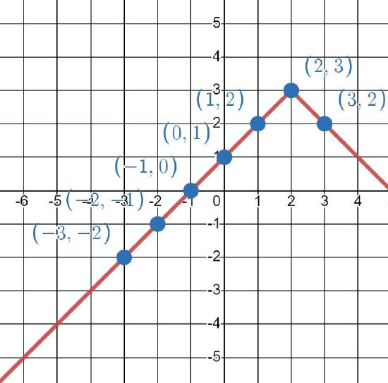\\ \hline \end{array}\)

Quadratic Functions

Our third family of functions we want to look at are the quadratic functions. These functions are the ones where the largest exponent appearing in the rule is a 2. That is, \(x\) is allowed to be squared or appear as just \(x\), but we can't have anything that looks like \(x^3\), \(x^4\), etc in the rule. The "parent" function for this family is

\(f(x) = x^2.\)

Similar to the absolute value function, this function has a graph that appears to have two branches reaching upward, since anything squared is positive, but it takes on more of a "U" shape since it curves smoothly around the base.

All quadratic functions have this same basic shape. However, just like the absolute value based functions, the graphs of quadratic functions may appear flipped over, stretched, or moved up and down. Let's check out some other examples of quadratic functions!

Our first example has been moved vertically.

Example \(\PageIndex{9}\)

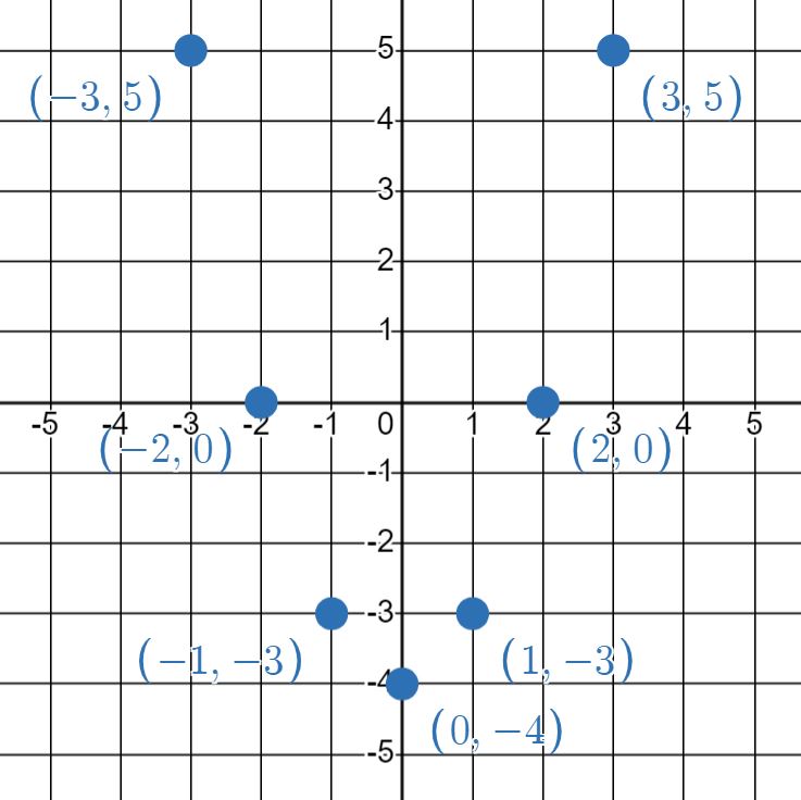
Graph the following quadratic function using a table: \(f(x) = x^2 - 4\)

Solution

We start by making a table with several points to plot. Since we are expecting a "U" shape, we should use some extra points:

\(\begin{array} {|c|c|}\hline x & f(x) & (x, f(x)) \\ \hline -3 & (-3)^2 - 4 = 5 & (-3, 5) \\ \hline -2 & (-2)^2 - 4 = 0 & (-2, 0) \\ \hline -1 & (-1)^2 - 4 = -3 & (-1, -3) \\ \hline 0 & 0^2 - 4 = -4 & (0, -4) \\ \hline 1 & 1^2 - 4 = -3 & (1, -3) \\ \hline 2 & 2^2 - 4 = 0 & (2, 0) \\ \hline 3 & 3^2 - 4 = 5 & (3, 5) \\ \hline \end{array}\)

Plot the points on a graph.

We connect the dots using a curved line, since quadratic functions all have a "U" shape, so the base of it should be rounded instead of being a corner.

Let's look at another example where the exponent 2 isn't directly attached to the \(x\). This still counts as a quadratic function because the exponent affects the \(x\) even though it is outside of parentheses! We will look at this in more detail in Section 4.

In this example, the graph has been moved horizontally.

Exercise \(\PageIndex{10}\)

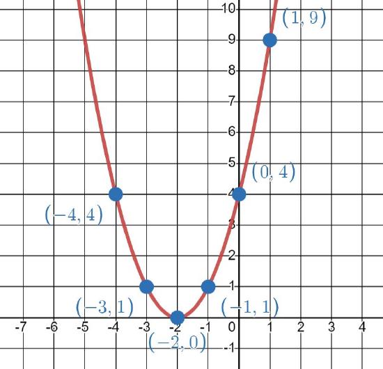
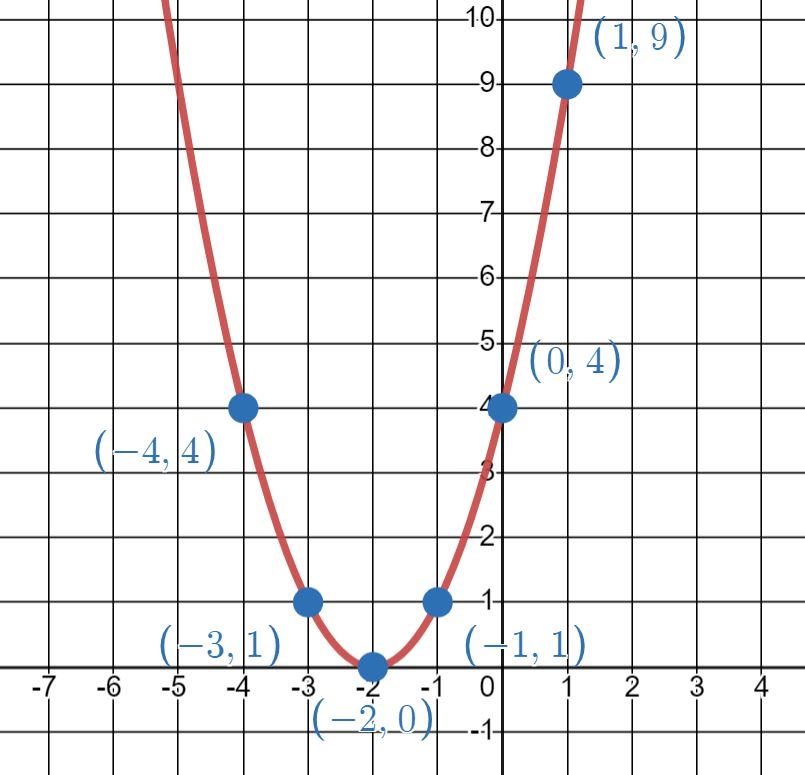
Graph the following quadratic function using a table: \(f(x) = (x + 2)^2\)

Answer

Notice that in this one, the points are a little "imbalanced", but since we know the general shape of the graph, we can be confident that the left side looks the same as the right side and we can complete the "U" shape in the sketch using that information.

Table	Graph
\(\begin{array} {|c|c|}\hline x & f(x) & (x, f(x)) \\ \hline -4 & (-4 + 2)^2 = (-2)^2 = 4 & (-4, 4) \\ \hline -3 & (-3 + 2)^2 = (-1)^2 = 1 & (-3, 1) \\ \hline -2 & (-2 + 2)^2 = 0^2 = 0 & (-2, 0) \\ \hline -1& (-1 + 2)^2 = 1^2 = 1 & (-1, 1) \\ \hline 0 & (0 + 2)^2 = 2^2 = 4 & (0, 4)\\ \hline 1& (1 + 2)^2 = 3^2 = 9 & (1, 9)\\ \hline \end{array}\)

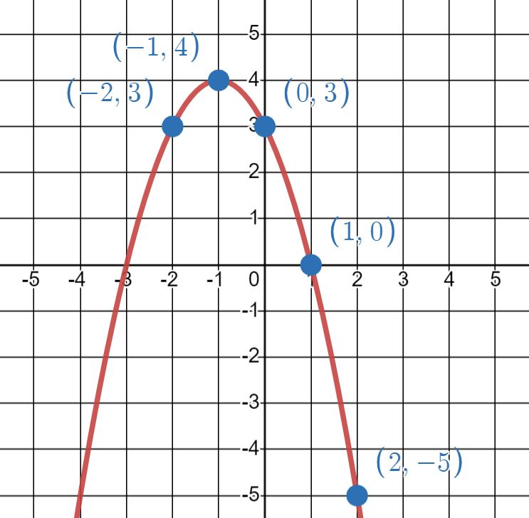
Our next example is another format for a quadratic that includes the \(x^2\), an \(x\) term, and a constant term. This graph has been moved horizontally, vertically, and flipped over!

Exercise \(\PageIndex{11}\)

Graph the following quadratic function using a table: \(f(x) = -x^2 - 2x + 3\)

Answer

Table	Graph
\(\begin{array} {|c|c|}\hline x & f(x) & (x, f(x)) \\ \hline -2 & -(-2)^2 - 2(-2) + 3 = 3 & (-2, 3) \\ \hline -1 & -(-1)^2 - 2(-1) + 3 = 4 & (-1, 4)\\ \hline 0 & -(0)^2 - 2(0) + 3 = 3 & (0, 3) \\ \hline 1 & -(1)^2 - 2(1) + 3 = 0 & (1, 0) \\ \hline 2 & -(2)^2 - 2(2) + 3 = -5 & (2, -5) 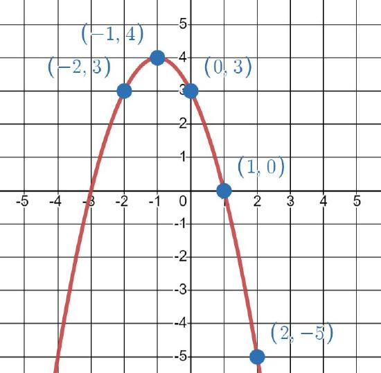\\ \hline \end{array}\)

Square root.

Square root functions are closely related to quadratic functions, because as you may have already noticed, square roots "undo" squaring a number, and vice versa, squaring a number "undoes" a square root. As a result, the square root family of functions have graphs that somewhat resemble the quadratic graphs with two notable exceptions -- 1) they're sideways and 2) it's only half the graph.

The "parent" functions for the square root family is

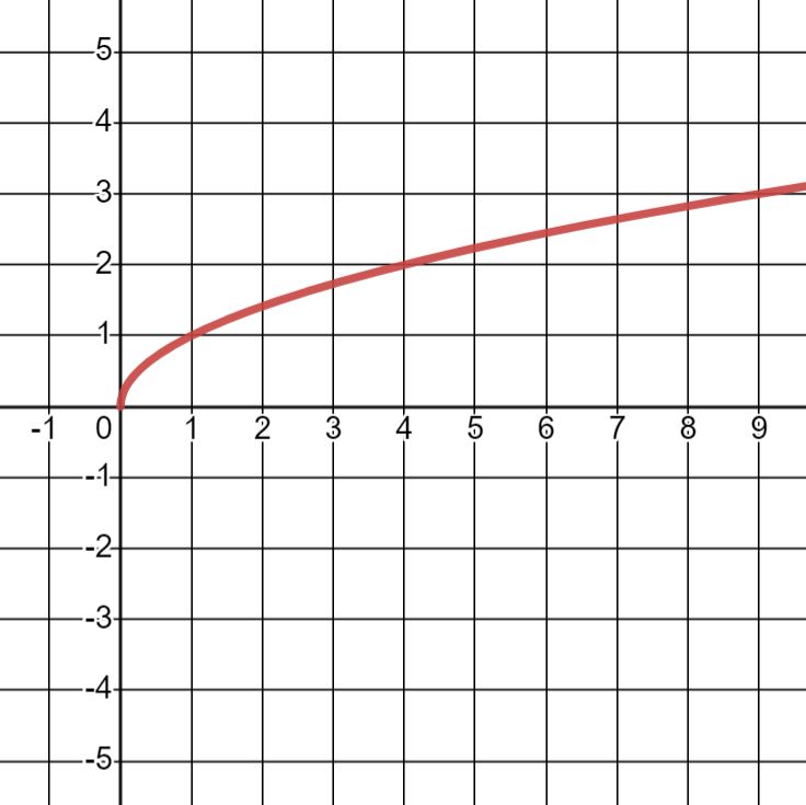
\(f(x) = \sqrt{x}.\)

Notice how the graph looks like half of the quadratic graph that's been turned on its side. The basic shape is a "swoosh", but just like with the previous families, other functions in this family may be modified so that their graph is flipped over vertically or horizontally, moved around, or stretched.

There are three really important things about the square root functions to point out.

1. Remember that when we take the square root of a number, we get both a positive and a negative answer. However, when we are thinking about square root as a function, we only want it to have ONE output, not two. In order for a square root to be considered a function, we only consider the positive results from square roots.
2. Since every squared real number produces a positive number, going the opposite direction with a square root means we cannot take the square root of a negative number and get a real number back. That is, when we are looking at square roots as a function, we only take the square roots of positive numbers or 0.
3. Always make the first point you graph the place where you are taking the square root of 0 to make sure the "swoosh" starts in the right place.

When graphing these types of functions, it's pretty common to wind up with decimals for outputs because the inputs may not always result in taking "nice" square roots. If we want, we can choose "convenient" numbers to plug in that will always cause us to take square roots of these "nice" numbers (e.g., 0, 1, 4, 9, 16, etc), or we can just deal with the decimals. It's entirely up to you!

Our first example has been moved horizontally.

Example \(\PageIndex{12}\)

Graph the following square root function using a table: \(f(x)=\sqrt{x + 1}\)

Solution

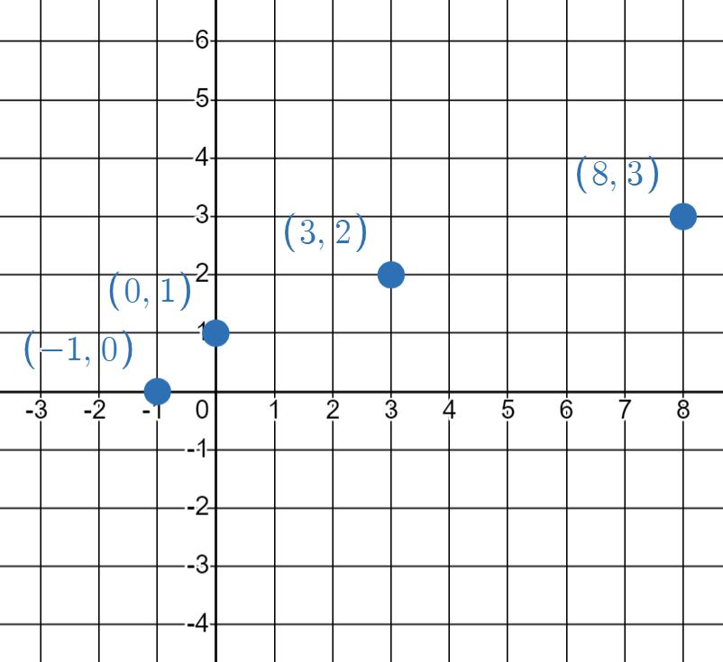
We first make the table with points to plot. Notice that since inside the square root is \(x + 1\), starting at \(x = -1\) is fine because \(-1 + 1 = 0\), which we are allowed to take the square root of! This will be the first point we want to include on the table. From here, we'd like to take square roots of the "nice" squared numbers 1, 4, and 9. So we want to plug in \(x = 0, 3,\) and 8.

\(\begin{array} {|c|c|}\hline x & f(x) & (x, f(x)) \\ \hline -1 & \sqrt{-1 + 1} = \sqrt{0} = 0 & (-1, 0) \\ \hline 0 & \sqrt{0 + 1} = \sqrt{1} = 1 & (0, 1) \\ \hline 3 & \sqrt{3 + 1} = \sqrt{4} = 2 & (3, 2) \\ \hline 8 & \sqrt{8 + 1} = \sqrt{9} = 3 & (8, 3) \\ \hline \end{array}\)

Now we plot the points.

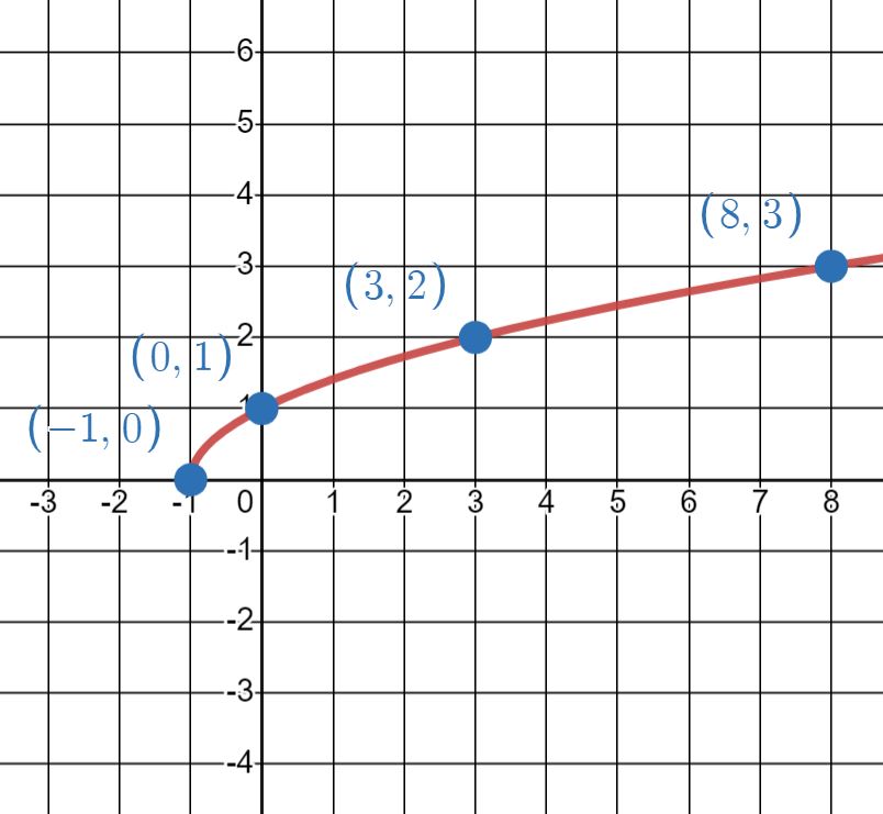
We complete the graph by knowing that it starts at (-1, 0), and then must follow the "swoosh" shape to the right.

Let's look at a version of the graph that has been moved around both horizontally and vertically.

Example \(\PageIndex{13}\)

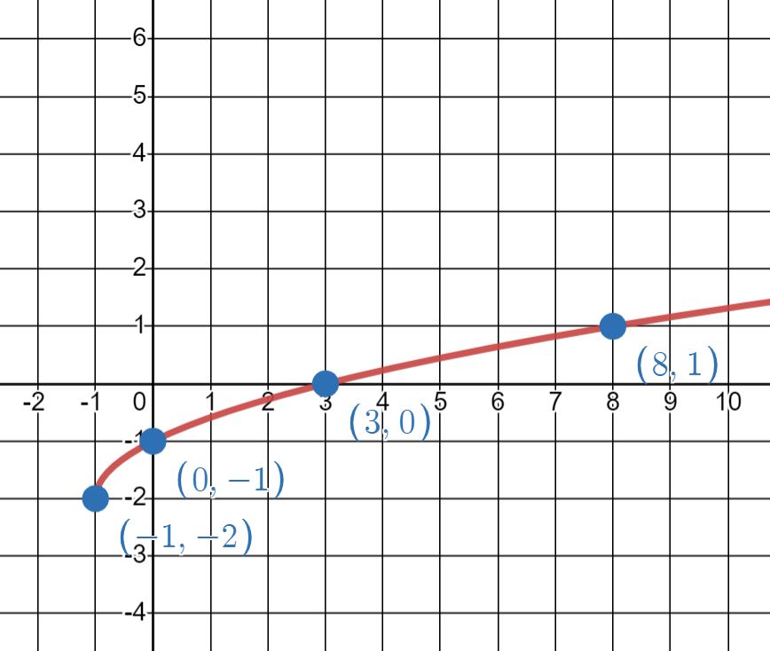
Graph \(f(x)=\sqrt{x+1}-2\) by plotting points.

Answer

In regards to the table, notice that once again since inside the square root is \(x + 1\), starting at \(x = -1\) is fine because \(-1 + 1 = 0\), which we are allowed to take the square root of! This will be the first point we want to include on the table. From here, we'd like to take square roots of the "nice" squared numbers 1, 4, and 9. So we want to plug in \(x = 0, 3,\) and 8.

Table	Graph
\(\begin{array} {|c|c|}\hline x & f(x) & (x, f(x)) \\ \hline -1 & \sqrt{-1 + 1} - 2 = \sqrt{0} - 2 = -2 & (-1, -2) \\ \hline 0 & \sqrt{0 + 1} - 2= \sqrt{1} - 2 = -1 & (0, -1) \\ \hline 3 & \sqrt{3 + 1} - 2= \sqrt{4} - 2= 0& (3, 0) \\ \hline 8 & \sqrt{8 + 1} - 2= \sqrt{9} - 2= 1 & (8, 1) \\ \hline \end{array}\)

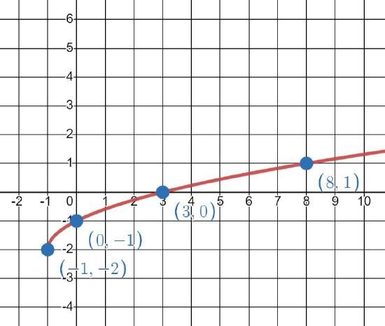
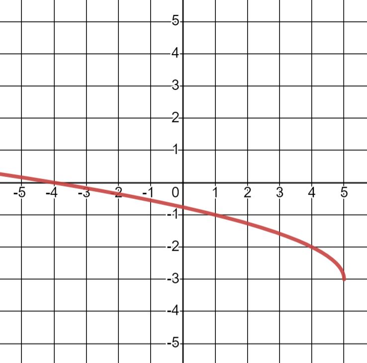
Finally, let's look at an example where the square root "swoosh" has been moved horizontally, vertically, and flipped over.

Exercise \(\PageIndex{14}\)

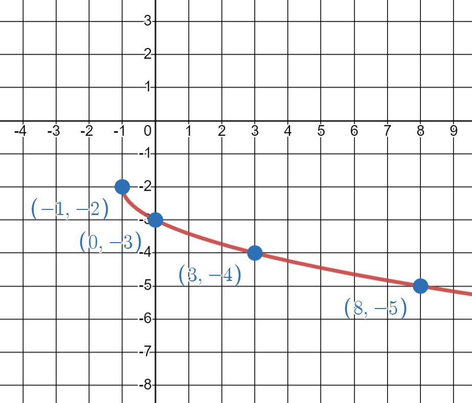
Graph the following square root function using a table: \(f(x) = -\sqrt{x+1}-2\)

Answer

Table	Graph
\(\begin{array} {|c|c|}\hline x & f(x) & (x, f(x)) \\ \hline -1 & -\sqrt{-1 + 1} - 2 = -\sqrt{0} - 2 = -2 & (-1, -2) \\ \hline 0 & -\sqrt{0 + 1} - 2= -\sqrt{1} - 2 = -3 & (0, -3) \\ \hline 3 & -\sqrt{3 + 1} - 2= -\sqrt{4} - 2= -4& (3, -4) \\ \hline 8 & -\sqrt{8 + 1} - 2= -\sqrt{9} - 2= -5 & (8, -5) \\ \hline \end{array}\)

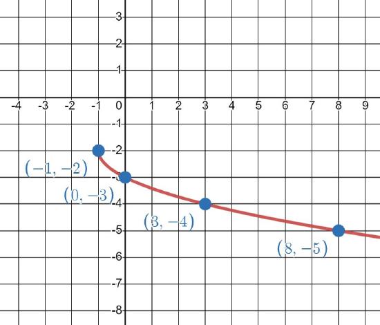
Quotient graph

Our last family of functions is the quotient function. Quotient is just the math way of saying division, and these functions get their name from dividing by the input \(x\). The parent function for this family is

\(f(x) = \frac{1}{x}.\)

The graph of \(f(x) = \frac{1}{x}\) is really distinct because unlike the previous functions, its graph has two pieces, and not just one.

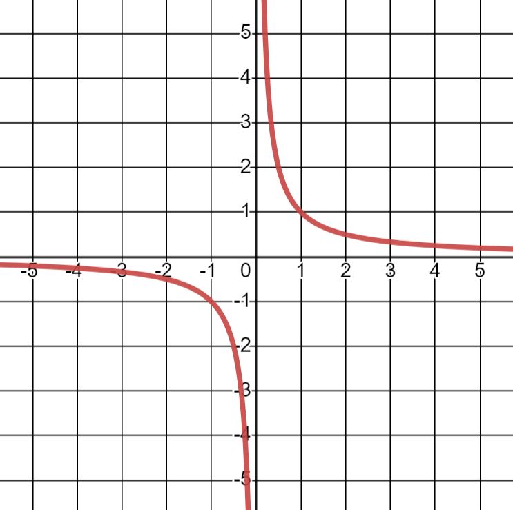
The two pieces show up because if you'll remember, we cannot divide by \(x = 0\). This means there is a gap in the horizontal direction whenever 0 may appear in the denominator of one of these functions. There is also a gap in the vertical direction due to the fact that nothing we divide by can ever cause the entire function to equal zero. These gaps have a special name:

Definition: Asymptote

A horizontal asymptote is the horizontal line that the graph approaches as \(x\to \pm\infty\).

A vertical asymptote is the vertical line that the graph approaches as the denominator approaches 0.

Let's look at some other examples of functions that are in this family, starting with one that has been moved around vertically.

Example \(\PageIndex{15}\)

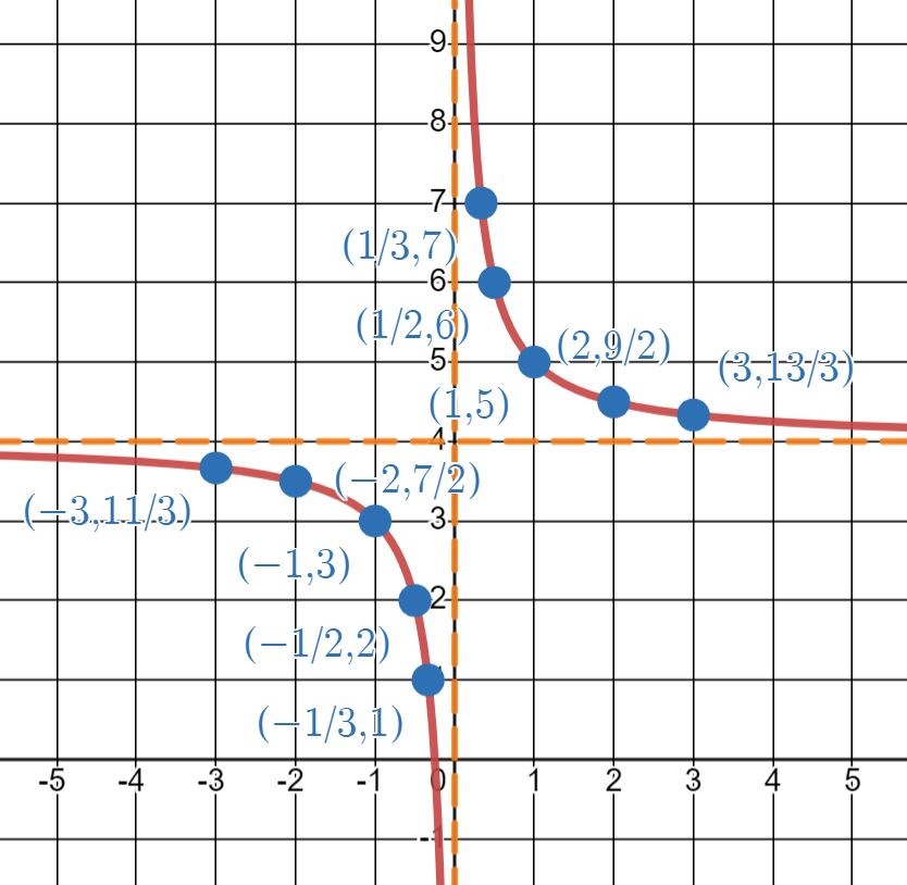
Graph the following quotient function using a table: \(f(x) = \frac{1}{x} + 4\)

Solution

First, we make a table. With these kinds of functions, fractions will be a necessity to understand their general shape! Also, since there are two pieces to the graph, we want to make sure to use enough points to capture both pieces!

\(\begin{array} {|c|c|}\hline x & f(x) & (x, f(x)) \\ \hline -3 & \frac{1}{-3} + 4 = -\frac{1}{3} + 4 = \frac{11}{3}& (-3, \frac{11}{3})\\ \hline -2 & \frac{1}{-2} + 4 = -\frac{1}{2} + 4 = \frac{7}{2}& (-2, \frac{7}{2})\\ \hline -1 & \frac{1}{-1} + 4 = -1 + 4 = 3& (-1, 3)\\ \hline -\frac{1}{2} & \frac{1}{-1/2} + 4 = -2 + 4 = 2& (-\frac{1}{2}, 2) \\ \hline -\frac{1}{3} & \frac{1}{-1/3} + 4 = -3 + 4 = 1& (-\frac{1}{3}, 1)\\ \hline 0 & ??? + 4 =???& \text{ draw vertical gap line at \(x = 0\)}\\ \hline \frac{1}{3} & \frac{1}{1/3} + 4 = 3 + 4 = 7& (\frac{1}{3}, 7)\\ \hline \frac{1}{2} & \frac{1}{1/2} + 4 = 2 + 4 = 6& (\frac{1}{2}, 6) \\ \hline 1 & \frac{1}{1} + 4 = 1 + 4 = 3& (1, 5)\\ \hline 2 & \frac{1}{2} + 4 = \frac{1}{2} + 4 = \frac{9}{2}& (2, \frac{9}{2})\\ \hline 3 & \frac{1}{3} + 4 = \frac{1}{3} + 4 = \frac{13}{3}& (3, \frac{13}{3})\\ \hline \end{array}\)

The vertical asymptote goes at the \(x\) value that make the denominator zero. In this example, the denomator is zero when \(x = 0\), so we can add a dashed line at \(x = 0\) to remind ourselves we don't want to graph there.

The horizontal asymptote goes at the \(y\) value that each part of the graph are approaching. In this example, each half of the graph will approach \(y = 4\), so we can add a dashed line at \(y = 4\) to remind ourselves that we don't want to graph there.

Now we plot the points and asymptotes.

When we add the lines, we have the two curves, where the curves follow the points AND asymptotes.

We can shift this graph too. Lets shift it in the same way as we did with \(\sqrt{x}\).

Example \(\PageIndex{16}\)

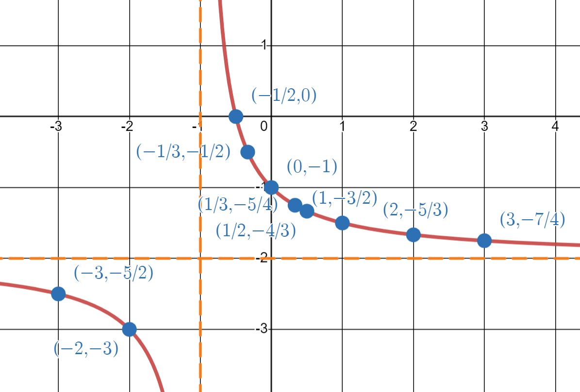
Graph \(f(x)=\frac{1}{x+1}-2\) by plotting points.

Answer

Table

Graph

\(\begin{array} {|c|c|}\hline x & f(x) & (x, f(x)) \\ \hline -3 & \frac{1}{-3 + 1} - 2 = \frac{1}{-2} - 2 = \frac{-5}{2}& (-3, \frac{-5}{2})\\ \hline -2 & \frac{1}{-2 + 1} - 2 = \frac{1}{-1} - 2 = -3& (-2, -3)\\ \hline -1 & \frac{1}{-1 + 1} - 2 = ??? - 2 = ???& \text{ draw vertical gap line at \(x = -1\) }\\ \hline -\frac{1}{2} & \frac{1}{-1/2 + 1} - 2 = \frac{1}{1/2} - 2 = 0& (-\frac{1}{2}, 0) \\ \hline -\frac{1}{3} & \frac{1}{-1/3 + 1} - 2 = \frac{3}{2} - 2 = -\frac{1}{2}& (-\frac{1}{3}, -\frac{1}{2})\\ \hline 0 & \frac{1}{0 + 1} - 2 = 1 - 2 = -1 & (0, -1)\\ \hline \frac{1}{3} & \frac{1}{1/3 + 1} - 2 = \frac{3}{4} - 2 = -\frac{5}{4}& (\frac{1}{3}, -\frac{5}{4})\\ \hline \frac{1}{2} & \frac{1}{1/2 + 1} - 2 = \frac{2}{3} - 2 = -\frac{4}{3}& (\frac{1}{2}, -\frac{4}{3}) \\ \hline 1 & \frac{1}{1 + 1} - 2 = \frac{1}{2} - 2 = -\frac{3}{2}& (1, -\frac{3}{2})\\ \hline 2 & \frac{1}{2 + 1} - 2 = \frac{1}{2 + 1} - 2 = -\frac{5}{3}& (2, -\frac{5}{3})\\ \hline 3 & \frac{1}{3 + 1} - 2= \frac{1}{4} - 2 = -\frac{7}{4}& (3, -\frac{7}{4})\\ \hline \end{array}\)

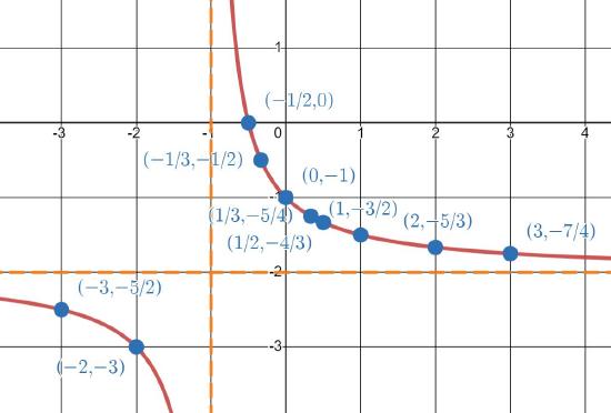
Here we see that x=-1 is a vertical asymptote and y=-2 is a horizontal asymptote.

Identifying Graphs of Families of Functions

The main point of this section is to highlight the fact that graphs of certain functions always appear a certain way, dependent on the key feature present in the rule. Being able to identify which type of graph goes with which type of function can really help your intuition for what is happening in the long run in this class! So we conclude with some examples of how you can match a function to its graph and vice versa simply based on what type of function it is.

Example \(\PageIndex{17}\)

Identify what family of functions each graph belongs to and then match it to the correct function.

Graph	Function
a.	1. \(f(x) = 2x - 3\)
b.	2. \(f(x) = \frac{1}{x + 3}\)
c.	3. \(f(x) = -(x - 4)^2 + 3\)
d.	4. \(f(x) = 2|x - 2| + 4\)

Solution

1. The first graph represents an absolute value function. Therefore, it must have come from the function \(f(x) = 2|x - 2| + 4\), option (4).
2. The second graph represents a quotient function. Therefore, it must have come from the function \(f(x) = \frac{1}{x + 3}\), option (2).
3. The third graph represents a linear function. Therefore, it must have come from the function \(f(x) = 2x - 3\), option (1).
4. The final graph represents a quadratic function. Therefore, it must have come from the function \(f(x) = -(x - 4)^2 + 3\), option (3).

Try it out on your own!

Exercise \(\PageIndex{18}\)

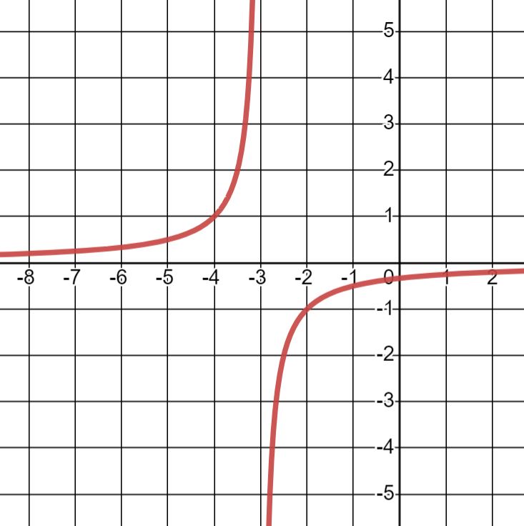
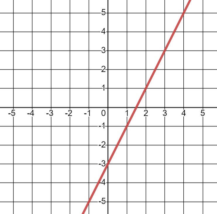
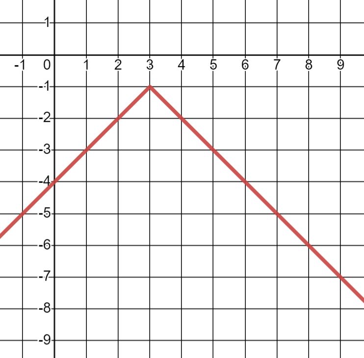
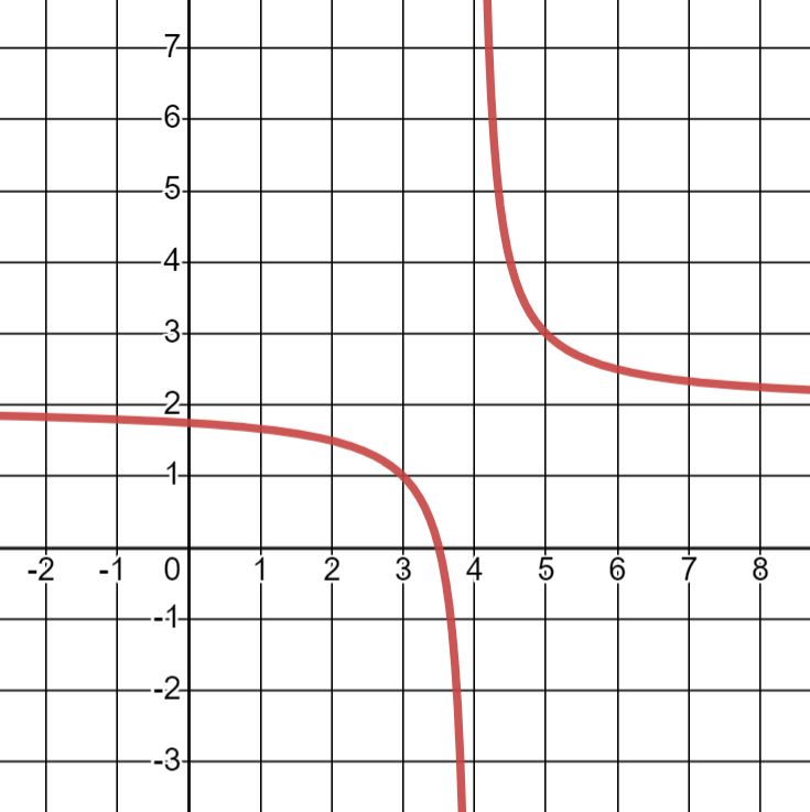
Identify what family of functions each graph belongs to and then match it to the correct function.

Graph	Function
a.	1. \(f(x) = -|x -3| - 1\)
b.	2. \(f(x) = -2\)
c.	3. \(f(x) = \frac{1}{x - 4} + 2\)
d.	4. \(f(x) = \sqrt{-x + 5} - 3\)

Answer

1. The first graph represents a linear function. Therefore, it must have come from the function \(f(x) = -2\), option (2).
2. The second graph represents an absolute value function. Therefore, it must have come from the function \(f(x) = -|x -3| - 1\), option (1).
3. The third graph represents a quotient function. Therefore, it must have come from the function \(f(x) = \frac{1}{x - 4} + 2\), option (3).
4. The final graph represents a square root function. Therefore, it must have come from the function \(f(x) = \sqrt{-x + 5} - 3\), option (4).

Key Concepts

Functions can be grouped into families according to the main features in their rules. These main features control how functions appear when graphed, and therefore functions of the same family all have graphs with the same basic shape.

Family	Parent Function	Basic Shape (graph of parent function)
Linear	\(f(x) = x\)
Absolute Value	\(f(x) = |x|\)
Quadratic	\(f(x) = x^2\)
Square Root	\(f(x) = \sqrt{x}\)
Quotient	\(f(x) = \frac{1}{x}\)