
4.11: Orthogonality


- Last updated
- Feb 16, 2025
- Save as PDF

( \newcommand{\kernel}{\mathrm{null}\,}\)
- Determine if a given set is orthogonal or orthonormal.
- Determine if a given matrix is orthogonal.
- Given a linearly independent set, use the Gram-Schmidt Process to find corresponding orthogonal and orthonormal sets.
- Find the orthogonal projection of a vector onto a subspace.
- Find the least squares approximation for a collection of points.
In this section, we examine what it means for vectors (and sets of vectors) to be orthogonal and orthonormal. First, it is necessary to review some important concepts. You may recall the definitions for the span of a set of vectors and a linear independent set of vectors. We include the definitions and examples here for convenience.
The collection of all linear combinations of a set of vectors
We call a collection of the form
Consider the following example.
Describe the span of the vectors
Solution
You can see that any linear combination of the vectors
Moreover every vector in the
Thus span
The span of a set of a vectors in
Another important property of sets of vectors is called linear independence.
A set of non-zero vectors
Here is an example.
Consider vectors
Solution
We already verified in Example
In terms of spanning, a set of vectors is linearly independent if it does not contain unnecessary vectors. In the previous example you can see that the vector
We can also determine if a set of vectors is linearly independent by examining linear combinations. A set of vectors is linearly independent if and only if whenever a linear combination of these vectors equals zero, it follows that all the coefficients equal zero. It is a good exercise to verify this equivalence, and this latter condition is often used as the (equivalent) definition of linear independence.
If a subspace is spanned by a linearly independent set of vectors, then we say that it is a basis for the subspace.
Let
is linearly independent
Thus the set of vectors
Recall from the properties of the dot product of vectors that two vectors
Let
Solution
Write
Then
Since
We can now discuss what is meant by an orthogonal set of vectors.
Let
If we have an orthogonal set of vectors and normalize each vector so they have length 1, the resulting set is called an orthonormal set of vectors. They can be described as follows.
A set of vectors,
Note that all orthonormal sets are orthogonal, but the reverse is not necessarily true since the vectors may not be normalized. In order to normalize the vectors, we simply need divide each one by its length.
Below is a video on orthogonal and orthonormal sets of vectors.
Normalizing an orthogonal set is the process of turning an orthogonal (but not orthonormal) set into an orthonormal set. If
We illustrate this concept in the following example.
Consider the set of vectors given by
Solution
One easily verifies that
Thus to find a corresponding orthonormal set, we simply need to normalize each vector. We will write
Similarly,
Therefore the corresponding orthonormal set is
You can verify that this set is orthogonal.
Consider an orthogonal set of vectors in
Let
- Proof
-
To show it is a linearly independent set, suppose a linear combination of these vectors equals
, such as: We need to show that all and obtain the following. Now since the set is orthogonal,
Since the set is orthogonal, we know that
was chosen arbitrarily, the set is linearly independent. Finally since
and therefore forms a basis of .
If an orthogonal set is a basis for a subspace, we call this an orthogonal basis. Similarly, if an orthonormal set is a basis, we call this an orthonormal basis.
We conclude this section with a discussion of Fourier expansions. Given any orthogonal basis
Let
This expression is called the Fourier expansion of
Consider the following example.
Let
Then
Compute the Fourier expansion of
Solution
Since
That is:
We readily compute:
Therefore,
Orthogonal Matrices
Recall that the process to find the inverse of a matrix was often cumbersome. In contrast, it was very easy to take the transpose of a matrix. Luckily for some special matrices, the transpose equals the inverse. When an
The precise definition is as follows.
A real
Note since
Consider the following example.
Orthogonal Matrix Show the matrix
Solution
All we need to do is verify (one of the equations from) the requirements of Definition
Since
Here is another example.
Orthogonal Matrix Let
Solution
Again the answer is yes and this can be verified simply by showing that
When we say that
In words, the product of the
More succinctly, this states that if
We will say that the columns form an orthonormal set of vectors, and similarly for the rows. Thus a matrix is orthogonal if its rows (or columns) form an orthonormal set of vectors. Notice that the convention is to call such a matrix orthogonal rather than orthonormal (although this may make more sense!).
The rows of an
- Proof
-
Recall from Theorem
that an orthonormal set is linearly independent and forms a basis for its span. Since the rows of an linearly independent vectors, and it follows that their span equals . Therefore these vectors form an orthonormal basis for . Suppose now that we have an orthonormal basis for
. Since the basis will contain vectors, these can be used to construct an
Consider the following proposition.
Det Suppose
- Proof
-
This result follows from the properties of determinants. Recall that for any matrix
, is orthogonal, then: Therefore
Orthogonal matrices are divided into two classes, proper and improper. The proper orthogonal matrices are those whose determinant equals 1 and the improper ones are those whose determinant equals
We conclude this section with two useful properties of orthogonal matrices.
Suppose
Solution
First we examine the product
Next we show that
Gram-Schmidt Process
The Gram-Schmidt process is an algorithm to transform a set of vectors into an orthonormal set spanning the same subspace, that is generating the same collection of linear combinations (see Definition 9.2.2).
The goal of the Gram-Schmidt process is to take a linearly independent set of vectors and transform it into an orthonormal set with the same span. The first objective is to construct an orthogonal set of vectors with the same span, since from there an orthonormal set can be obtained by simply dividing each vector by its length.
Process
Let
I: Construct a new set of vectors
II: Now let
Then
is an orthogonal set. is an orthonormal set.
Solution
The full proof of this algorithm is beyond this material, however here is an indication of the arguments.
To show that
Then in a similar fashion you show that
Finally defining
Below is a video on the Gram Schmidt process.

Consider the following example.
Span
Consider the set of vectors
Use the Gram-Schmidt algorithm to find an orthonormal set of vectors
Solution
We already remarked that the set of vectors in
Now to normalize simply let
You can verify that
In this example, we began with a linearly independent set and found an orthonormal set of vectors which had the same span. It turns out that if we start with a basis of a subspace and apply the Gram-Schmidt algorithm, the result will be an orthogonal basis of the same subspace. We examine this in the following example.
Basis
Let
Solution
First
Next,
Finally,
Therefore,
Below is another video on the Gram Schmidt process.

Orthogonal Projections
An important use of the Gram-Schmidt Process is in orthogonal projections, the focus of this section.
You may recall that a subspace of
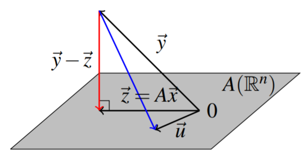
Suppose a point
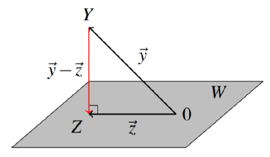
The vector
Projection
Let
Therefore, in order to find the orthogonal projection, we must first find an orthogonal basis for the subspace. Note that one could use an orthonormal basis, but it is not necessary in this case since as you can see above the normalization of each vector is included in the formula for the projection.
Below is a video on finding an orthogonal projection of a vector onto a line.
Below is a video on finding an orthogonal projection of a vector onto a plane.

Below is a video on finding an orthogonal projection of a vector onto a subspace of
Before we explore this further through an example, we show that the orthogonal projection does indeed yield a point
Theorem
Let
Then,
- Proof
-
First
is certainly a point in since it is in the span of a basis of . To show that
is the point in closest to , we wish to show that , and . Therefore these vectors are orthogonal to each other. By the Pythagorean Theorem, we have that This follows because Hence,
Consider the following example.
Projection
Let
Find the point in
Solution
We must first find an orthogonal basis for
We can thus write
Notice that this span is a basis of
Therefore an orthogonal basis of
We can now use this basis to find the orthogonal projection of the point
Therefore the point
Recall that the vector
Complement
Let
The orthogonal complement is defined as the set of all vectors which are orthogonal to all vectors in the original subspace. It turns out that it is sufficient that the vectors in the orthogonal complement be orthogonal to a spanning set of the original space.
Set
Let
The following proposition demonstrates that the orthogonal complement of a subspace is itself a subspace.
Complement
Let
Consider the following proposition.
The complement of
- Proof
-
Here,
is the zero vector of . Since Again, since
In the next example, we will look at how to find
Complement
Let
Solution
From Example
In order to find
Let
In order to satisfy
Both of these equations must be satisfied, so we have the following system of equations.
To solve, set up the augmented matrix.
Using Gaussian Elimination, we find that
The following results summarize the important properties of the orthogonal projection.
Projection
Let
- The position vector
of the point is given by
Consider the following example of this concept.
Vector
Let
Solution
We will first use the Gram-Schmidt Process to construct the orthogonal basis,
By Theorem
Consider the next example.
Vectors
Let
Find the point
Solution
From Theorem
Notice that since the above vectors already give an orthogonal basis for
Therefore the point in
Now, we need to write
The vector
Point
Find the point
Solution
The solution will proceed as follows.
- Find a basis
of the subspace of defined by the equation - Orthogonalize the basis
to get an orthogonal basis of . - Find the projection on
of the position vector of the point .
We now begin the solution.
gives general solution Let is linearly independent and is a basis of . - Use the Gram-Schmidt Process to get an orthogonal basis of
: Therefore . - To find the point
on closest to Therefore,
Least Squares Approximation
It should not be surprising to hear that many problems do not have a perfect solution, and in these cases the objective is always to try to do the best possible. For example what does one do if there are no solutions to a system of linear equations
We begin with a lemma.
Recall that we can form the image of an
Minimizers
Let
Choose
Then
We note a simple but useful observation.
Product
Let
- Proof
-
This follows from the definitions:
The next corollary gives the technique of least squares.
Equation
A specific value of
Note that
Consider the following example.
Find a least squares solution to the system
Solution
First, consider whether there exists a real solution. To do so, set up the augmnented matrix given by
It follows that there is no real solution to this system. Therefore we wish to find the least squares solution. The normal equations are
Consider another example.
Find a least squares solution to the system
Solution
First, consider whether there exists a real solution. To do so, set up the augmnented matrix given by
It follows that the system has a solution given by
The least squares solution is
An important application of Corollary
which is of the form
as small as possible. According to Theorem
Thus, computing
Solving this system of equations for
Consider the following example.
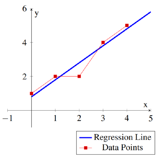
Find the least squares regression line
Solution
In this case we have
The least squares regression line for the set of data points is:
One could use this line to approximate other values for the data. For example for
The following diagram shows the data points and the corresponding regression line.
One could clearly do a least squares fit for curves of the form