9.3: Singular Points and the Method of Frobenius

Examples

While behavior of ODEs at singular points is more complicated, certain singular points are not especially difficult to solve. Let us look at some examples before giving a general method. We may be lucky and obtain a power series solution using the method of the previous section, but in general we may have to try other things.

Example $\PageIndex{1}$

Let us first look at a simple first order equation

$$2 x y' - y = 0 . \label{ex1eq1}$$

Note that $x=0$ is a singular point. If we only try to plug in

$$y = \sum_{k=0}^\infty a_k x^k ,\label{ex1eq2}$$

we obtain

$$\begin{align}\begin{aligned} 0 = 2 xy'-y &=2x \, \left( \sum_{k=1}^\infty k a_k x^{k-1} \right)-\left( \sum_{k=0}^\infty a_k x^k \right) \\ &=a_0 +\sum_{k=1}^\infty (2 k a_k - a_k) \, x^{k} . \end{aligned}\end{align} \label{ex1eq3}$$

First, $a_0 = 0$. Next, the only way to solve $0 = 2 k a_k - a_k = (2k-1) \, a_k$ for $k = 1,2,3,\dots$ is for $a_k = 0$ for all $k$. Therefore we only get the trivial solution $y=0$. We need a nonzero solution to get the general solution.

Let us try $y=x^r$ for some real number $r$. Consequently our solution---if we can find one---may only make sense for positive $x$. Then $y' = r x^{r-1}$. So

$$0 = 2 x y' - y = 2 x r x^{r-1} - x^r= (2r-1) x^r . \nonumber$$

Therefore $r= \dfrac{1}{2}$, or in other words $y = x^{1/2}$. Multiplying by a constant, the general solution for positive $x$ is

$$y = C x^{1/2} . \nonumber$$

If $C \not= 0$ then the derivative of the solution "blows up" at $x=0$ (the singular point). There is only one solution that is differentiable at $x=0$ and that's the trivial solution $y=0$.

Not every problem with a singular point has a solution of the form $y=x^r$, of course. But perhaps we can combine the methods. What we will do is to try a solution of the form

$$y = x^r f(x) \nonumber$$

where $f(x)$ is an analytic function.

Example $\PageIndex{2}$

Suppose that we have the equation

$$4 x^2 y'' - 4 x^2 y' + (1-2x)y = 0, \label{ex2eq1}$$

and again note that $x=0$ is a singular point. Let us try

$$y = x^r \sum_{k=0}^\infty a_k x^k = \sum_{k=0}^\infty a_k x^{k+r} , \label{ex2eq2}$$

where $r$ is a real number, not necessarily an integer. Again if such a solution exists, it may only exist for positive $x$. First let us find the derivatives

$$\begin{align} y' &= \sum_{k=0}^\infty (k+r)\, a_k x^{k+r-1} ,\nonumber \\ y'' &= \sum_{k=0}^\infty (k+r)\,(k+r-1)\, a_k x^{k+r-2} . \label{ex2eq3} \end{align}$$

Plugging Equations $\ref{ex2eq2}$ - $\ref{ex2eq3}$ into our original differential equation (Equation $\ref{ex2eq1}$) we obtain

$$\begin{align}\begin{aligned} 0 &= 4x^2y''-4x^2y'+(1-2x)y \\ &= 4x^2 \, \left( \sum_{k=0}^\infty (k+r)\,(k+r-1) \, a_k x^{k+r-2} \right)-4x^2 \, \left( \sum_{k=0}^\infty (k+r) \, a_k x^{k+r-1} \right)+(1-2x) \left( \sum_{k=0}^\infty a_k x^{k+r} \right) \\ &=\left( \sum_{k=0}^\infty 4 (k+r)\,(k+r-1) \, a_k x^{k+r} \right)-\left( \sum_{k=0}^\infty 4 (k+r) \, a_k x^{k+r+1} \right)+\left( \sum_{k=0}^\infty a_k x^{k+r} \right)-\left( \sum_{k=0}^\infty 2a_k x^{k+r+1} \right) \\ &=\left( \sum_{k=0}^\infty 4 (k+r)\,(k+r-1) \, a_k x^{k+r} \right)-\left( \sum_{k=1}^\infty 4 (k+r-1) \, a_{k-1} x^{k+r} \right)+\left( \sum_{k=0}^\infty a_k x^{k+r} \right)-\left( \sum_{k=1}^\infty 2a_{k-1} x^{k+r} \right)\\ &=4r(r-1) \, a_0 x^r + a_0 x^r +\sum_{k=1}^\infty \left( 4 (k+r)\,(k+r-1) \, a_k - 4 (k+r-1) \, a_{k-1}+a_k -2a_{k-1} \right) \, x^{k+r}\\ &=\left( 4r(r-1) + 1 \right) \, a_0 x^r +\sum_{k=1}^\infty\left( \left( 4 (k+r)\,(k+r-1) + 1 \right) \, a_k-\left( 4 (k+r-1) + 2 \right) \, a_{k-1} \right) \, x^{k+r} .\end{aligned}\end{align} \nonumber$$

To have a solution we must first have $\left( 4r(r-1) + 1 \right) \, a_0 = 0$. Supposing that $a_0 \not= 0$ we obtain

$$4r(r-1) + 1 = 0 . \nonumber$$

This equation is called the indicial equation. This particular indicial equation has a double root at $r = \dfrac{1}{2}$.

OK, so we know what $r$ has to be. That knowledge we obtained simply by looking at the coefficient of $x^r$. All other coefficients of $x^{k+r}$ also have to be zero so

$$\left( 4 (k+r)\,(k+r-1) + 1 \right) \, a_k- \left( 4 (k+r-1) + 2 \right) \, a_{k-1} = 0 . \nonumber$$

If we plug in $r=\dfrac{1}{2}$ and solve for $a_k$ we get

$$a_k=\dfrac{4 (k+\dfrac{1}{2}-1) + 2}{4 (k+\dfrac{1}{2})\,(k+\dfrac{1}{2}-1) + 1} \, a_{k-1}=\dfrac{1}{k} \, a_{k-1} . \nonumber$$

Let us set $a_0 = 1$. Then

$$a_1 = \dfrac{1}{1} a_0 = 1 , \qquad a_2 = \dfrac{1}{2} a_1 = \dfrac{1}{2} ,\qquad a_3 = \dfrac{1}{3} a_2 = \dfrac{1}{3 \cdot 2} ,\qquad a_4 = \dfrac{1}{4} a_3 = \dfrac{1}{4 \cdot 3 \cdot 2} , \qquad \dots \nonumber$$

Extrapolating, we notice that

$$a_k = \dfrac{1}{k(k-1)(k-2) \cdots 3 \cdot 2} = \dfrac{1}{k!} . \nonumber$$

In other words,

$$y =\sum_{k=0}^\infty a_k x^{k+r}=\sum_{k=0}^\infty \dfrac{1}{k!} x^{k+1/2}=x^{1/2} \sum_{k=0}^\infty \dfrac{1}{k!} x^{k}=x^{1/2}e^x . \nonumber$$

That was lucky! In general, we will not be able to write the series in terms of elementary functions. We have one solution, let us call it $y_1 = x^{1/2} e^x$. But what about a second solution? If we want a general solution, we need two linearly independent solutions. Picking $a_0$ to be a different constant only gets us a constant multiple of $y_1$, and we do not have any other $r$ to try; we only have one solution to the indicial equation. Well, there are powers of $x$ floating around and we are taking derivatives, perhaps the logarithm (the antiderivative of $x^{-1}$) is around as well. It turns out we want to try for another solution of the form

$$y_2 = \sum_{k=0}^\infty b_k x^{k+r} + (\ln x) y_1 , \nonumber$$

which in our case is

$$y_2 = \sum_{k=0}^\infty b_k x^{k+1/2} + (\ln x) x^{1/2} e^x . \nonumber$$

We now differentiate this equation, substitute into the differential equation and solve for $b_k$. A long computation ensues and we obtain some recursion relation for $b_k$. The reader can (and should) try this to obtain for example the first three terms

$$b_1 = b_0 -1 , \qquad b_2 = \dfrac{2b_1-1}{4} , \qquad b_3 = \dfrac{6b_2-1}{18} , \qquad \ldots \nonumber$$

We then fix $b_0$ and obtain a solution $y_2$. Then we write the general solution as $y = A y_1 + B y_2$.

Method of Frobenius

Before giving the general method, let us clarify when the method applies. Let

$$p(x) y'' + q(x) y' + r(x) y = 0 \nonumber$$

be an ODE. As before, if $p(x_0) = 0$, then $x_0$ is a singular point. If, furthermore, the limits

$$\lim_{x \to x_0} ~ (x-x_0) \dfrac{q(x)}{p(x)} \qquad \text{and} \qquad \lim_{x \to x_0} ~ (x-x_0)^2 \dfrac{r(x)}{p(x)} \nonumber$$

both exist and are finite, then we say that $x_0$ is a regular singular point.

Example $\PageIndex{3}$: Expansion around a regular singular point

Often, and for the rest of this section, $x_0 = 0$. Consider

$$x^2y'' + x(1+x)y' + (\pi+x^2)y = 0 . \nonumber$$

Write

$\begin{align}\begin{aligned} \lim_{x \to 0} ~x \dfrac{q(x)}{p(x)} &=\lim_{x \to 0} ~x \dfrac{x(1+x)}{x^2} = \lim_{x \to 0} ~(1+x) = 1 , \\ \lim_{x \to 0} ~x^2 \dfrac{r(x)}{p(x)} &=\lim_{x \to 0} ~x^2 \frac{(\pi+x^2)}{x^2} = \lim_{x \to 0} ~(\pi+x^2) = \pi \end{aligned}\end{align}. \nonumber$

So $x = 0$ is a regular singular point.

On the other hand if we make the slight change

$$x^2y'' + (1+x)y' + (\pi+x^2)y = 0 , \nonumber$$

then

$$\lim_{x \to 0} ~x \dfrac{q(x)}{p(x)} =\lim_{x \to 0} ~x \dfrac{(1+x)}{x^2} = \lim_{x \to 0} ~\dfrac{1+x}{x} =\text{DNE}. \nonumber$$

Here DNE stands for does not exist. The point $0$ is a singular point, but not a regular singular point.

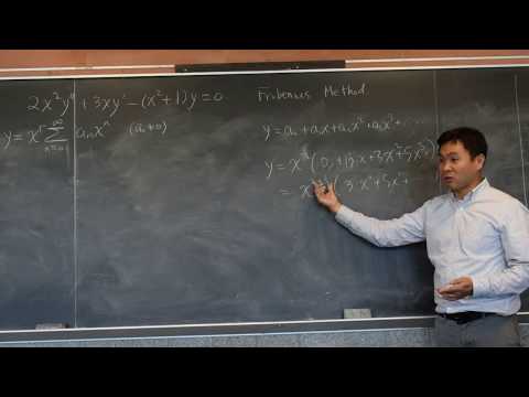
Below is part 1 of a video on the method of Frobenius.

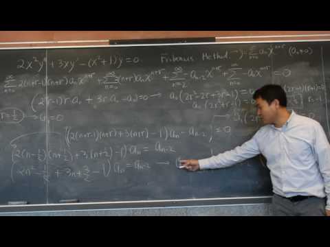
Below is part 2 of a video on the method of Frobenius.

Let us now discuss the general Method of Frobenius$^{1}$. Let us only consider the method at the point $x=0$ for simplicity. The main idea is the following theorem.

Theorem $\PageIndex{1}$

Method of Frobenius

Suppose that

$$\label{eq:26} p(x) y'' + q(x) y' + r(x) y = 0$$

has a regular singular point at $x=0$, then there exists at least one solution of the form

$$y = x^r \sum_{k=0}^\infty a_k x^k . \nonumber$$

A solution of this form is called a Frobenius-type solution.

The method usually breaks down like this.

1. We seek a Frobenius-type solution of the form $$y = \sum_{k=0}^\infty a_k x^{k+r} . \nonumber$$ We plug this $y$ into equation $\eqref{eq:26}$. We collect terms and write everything as a single series.
2. The obtained series must be zero. Setting the first coefficient (usually the coefficient of $x^r$) in the series to zero we obtain the indicial equation, which is a quadratic polynomial in $r$.
3. If the indicial equation has two real roots $r_1$ and $r_2$ such that $r_1 - r_2$ is not an integer, then we have two linearly independent Frobenius-type solutions. Using the first root, we plug in $$y_1 = x^{r_1} \sum_{k=0}^\infty a_k x^{k} , \nonumber$$ and we solve for all $a_k$ to obtain the first solution. Then using the second root, we plug in $$y_2 = x^{r_2} \sum_{k=0}^\infty b_k x^{k} , \nonumber$$ and solve for all $b_k$ to obtain the second solution.
4. If the indicial equation has a doubled root $r$, then there we find one solution $$y_1 = x^{r} \sum_{k=0}^\infty a_k x^{k} , \nonumber$$ and then we obtain a new solution by plugging $$y_2 = x^{r} \sum_{k=0}^\infty b_k x^{k} + (\ln x) y_1 , \nonumber$$ into Equation $\eqref{eq:26}$ and solving for the constants $b_k$.
5. If the indicial equation has two real roots such that $r_1-r_2$ is an integer, then one solution is $$y_1 = x^{r_1} \sum_{k=0}^\infty a_k x^{k} , \nonumber$$ and the second linearly independent solution is of the form $$y_2 = x^{r_2} \sum_{k=0}^\infty b_k x^{k} + C (\ln x) y_1 , \nonumber$$ where we plug $y_2$ into $\eqref{eq:26}$ and solve for the constants $b_k$ and $C$.
6. Finally, if the indicial equation has complex roots, then solving for $a_k$ in the solution $$y = x^{r_1} \sum_{k=0}^\infty a_k x^{k} \nonumber$$ results in a complex-valued function---all the $a_k$ are complex numbers. We obtain our two linearly independent solutions$^{2}$ by taking the real and imaginary parts of $y$.

The main idea is to find at least one Frobenius-type solution. If we are lucky and find two, we are done. If we only get one, we either use the ideas above or even a different method such as reduction of order (Exercise 2.1.8) to obtain a second solution.

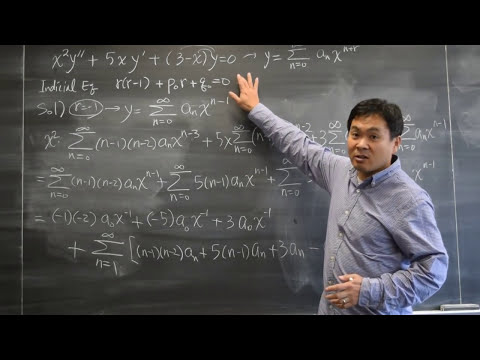
Below is a video on using the method of Frobenious to solve a differential equation.

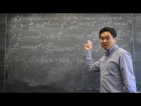
Below is another video on using the method of Frobenious to solve a differential equation.

Bessel Functions

An important class of functions that arises commonly in physics are the Bessel functions$^{3}$. For example, these functions appear when solving the wave equation in two and three dimensions. First we have Bessel's equation of order $p$:

$$x^2 y'' + xy' + \left(x^2 - p^2\right)y = 0 . \nonumber$$

We allow $p$ to be any number, not just an integer, although integers and multiples of $\dfrac{1}{2}$ are most important in applications. When we plug

$$y = \sum_{k=0}^\infty a_k x^{k+r} \nonumber$$

into Bessel's equation of order $p$ we obtain the indicial equation

$$r(r-1)+r-p^2 = (r-p)(r+p) = 0 . \nonumber$$

Therefore we obtain two roots $r_1 = p$ and $r_2 = -p$. If $p$ is not an integer following the method of Frobenius and setting $a_0 = 1$, we obtain linearly independent solutions of the form

$$\begin{align}\begin{aligned} y_1 &= x^p \sum_{k=0}^{\infty} \dfrac{(-1)^k x^{2k}}{2^{2k}k!(k+p)(k-1+p) \cdots (2+p)(1+p)}, \\ y_2 &= x^{-p} \sum_{k=0}^{\infty} \dfrac{(-1)^k x^{2k}}{2^{2k}k!(k-p)(k-1-p) \cdots (2-p)(1-p)}.\end{aligned}\end{align} \nonumber$$

Exercise $\PageIndex{1}$

1. Verify that the indicial equation of Bessel's equation of order $p$ is $(r-p)(r+p)=0$.
2. Suppose that $p$ is not an integer. Carry out the computation to obtain the solutions $y_1$ and $y_2$ above.

Bessel functions will be convenient constant multiples of $y_1$ and $y_2$. First we must define the gamma function

$$\Gamma(x) = \int_0^\infty t^{x-1} e^{-t} \, dt . \nonumber$$

Notice that $\Gamma(1) = 1$. The gamma function also has a wonderful property

$$\Gamma(x+1) = x \Gamma(x) . \nonumber$$

From this property, one can show that $\Gamma(n) = (n-1)!$ when $n$ is an integer, so the gamma function is a continuous version of the factorial. We compute:

$$\begin{align}\begin{aligned} \Gamma(k+p+1)=(k+p)(k-1+p)\cdots (2+p)(1+p) \Gamma(1+p) ,\\ \Gamma(k-p+1)=(k-p)(k-1-p)\cdots (2-p)(1-p) \Gamma(1-p) .\end{aligned}\end{align} \nonumber$$

Exercise $\PageIndex{2}$

Verify the above identities using $\Gamma(x+1) = x \Gamma(x)$.

We define the Bessel functions of the first kind of order $p$ and $-p$ as

$$\begin{align}\begin{aligned} J_p(x) &= \dfrac{1}{2^p\Gamma(1+p)} y_1=\sum_{k=0}^\infty \dfrac{{(-1)}^k}{k! \Gamma(k+p+1)}{\left(\dfrac{x}{2}\right)}^{2k+p} , \\ J_{-p}(x) &= \dfrac{1}{2^{-p}\Gamma(1-p)} y_2=\sum_{k=0}^\infty \dfrac{{(-1)}^k}{k! \Gamma(k-p+1)}{\left(\dfrac{x}{2}\right)}^{2k-p} .\end{aligned}\end{align} \nonumber$$

As these are constant multiples of the solutions we found above, these are both solutions to Bessel's equation of order $p$. The constants are picked for convenience.

When $p$ is not an integer, $J_p$ and $J_{-p}$ are linearly independent. When $n$ is an integer we obtain

$$J_n(x) =\sum_{k=0}^\infty \dfrac{{(-1)}^k}{k! (k+n)!}{\left(\dfrac{x}{2}\right)}^{2k+n} . \nonumber$$

In this case it turns out that

$$J_n(x) = {(-1)}^nJ_{-n}(x) , \nonumber$$

and so we do not obtain a second linearly independent solution. The other solution is the so-called Bessel function of second kind. These make sense only for integer orders $n$ and are defined as limits of linear combinations of $J_p(x)$ and $J_{-p}(x)$ as $p$ approaches $n$ in the following way:

$$Y_n(x) = \lim_{p\to n} \dfrac{\cos(p \pi) J_p(x) - J_{-p}(x)}{\sin(p \pi)} . \nonumber$$

As each linear combination of $J_p(x)$ and $J_{-p}(x)$ is a solution to Bessel's equation of order $p$, then as we take the limit as $p$ goes to $n$, $Y_n(x)$ is a solution to Bessel's equation of order $n$. It also turns out that $Y_n(x)$ and $J_n(x)$ are linearly independent. Therefore when $n$ is an integer, we have the general solution to Bessel's equation of order $n$

$$y = A J_n(x) + B Y_n(x) , \nonumber$$

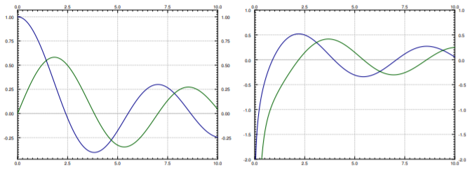
for arbitrary constants $A$ and $B$. Note that $Y_n(x)$ goes to negative infinity at $x=0$. Many mathematical software packages have these functions $J_n(x)$ and $Y_n(x)$ defined, so they can be used just like say $\sin(x)$ and $\cos(x)$. In fact, they have some similar properties. For example, $-J_1(x)$ is a derivative of $J_0(x)$, and in general the derivative of $J_n(x)$ can be written as a linear combination of $J_{n-1}(x)$ and $J_{n+1}(x)$. Furthermore, these functions oscillate, although they are not periodic. See Figure $\PageIndex{1}$ for graphs of Bessel functions.

Figure $\PageIndex{1}$: Plot of the $J_{0}(x)$ and $J_{1}(x)$ in the first graph and $Y_{0}(x)$ and $Y_{1}(x)$ in the second graph.

Example $\PageIndex{4}$: Using Bessel functions to Solve a ODE

Other equations can sometimes be solved in terms of the Bessel functions. For example, given a positive constant $\lambda$,

$$x y'' + y' + \lambda^2 x y = 0 , \nonumber$$

can be changed to $x^2 y'' + x y' + \lambda^2 x^2 y = 0$. Then changing variables $t = \lambda x$ we obtain via chain rule the equation in $y$ and $t$:

$$t^2 y'' + t y' + t^2 y = 0 , \nonumber$$

which can be recognized as Bessel's equation of order 0. Therefore the general solution is $y(t) = A J_0(t) + B Y_0(t)$, or in terms of $x$:

$$y = A J_0(\lambda x) + B Y_0(\lambda x) . \nonumber$$

This equation comes up for example when finding fundamental modes of vibration of a circular drum, but we digress.

Footnotes

[1] Named after the German mathematician Ferdinand Georg Frobenius (1849 – 1917).

[2] See Joseph L. Neuringera, The Frobenius method for complex roots of the indicial equation, International Journal of Mathematical Education in Science and Technology, Volume 9, Issue 1, 1978, 71–77.

[3] Named after the German astronomer and mathematician Friedrich Wilhelm Bessel (1784 – 1846).