Ellipses

Last updated
Save as PDF

Page ID: 221331

$ \newcommand{\vecs}[1]{\overset { \scriptstyle \rightharpoonup} {\mathbf{#1}} } $

$ \newcommand{\vecd}[1]{\overset{-\!-\!\rightharpoonup}{\vphantom{a}\smash {#1}}} $

$ \newcommand{\dsum}{\displaystyle\sum\limits} $

$ \newcommand{\dint}{\displaystyle\int\limits} $

$ \newcommand{\dlim}{\displaystyle\lim\limits} $

$ \newcommand{\id}{\mathrm{id}}$ $ \newcommand{\Span}{\mathrm{span}}$

( \newcommand{\kernel}{\mathrm{null}\,}\) $ \newcommand{\range}{\mathrm{range}\,}$

$ \newcommand{\RealPart}{\mathrm{Re}}$ $ \newcommand{\ImaginaryPart}{\mathrm{Im}}$

$ \newcommand{\Argument}{\mathrm{Arg}}$ $ \newcommand{\norm}[1]{\| #1 \|}$

$ \newcommand{\inner}[2]{\langle #1, #2 \rangle}$

$ \newcommand{\Span}{\mathrm{span}}$

$ \newcommand{\id}{\mathrm{id}}$

$ \newcommand{\Span}{\mathrm{span}}$

$ \newcommand{\kernel}{\mathrm{null}\,}$

$ \newcommand{\range}{\mathrm{range}\,}$

$ \newcommand{\RealPart}{\mathrm{Re}}$

$ \newcommand{\ImaginaryPart}{\mathrm{Im}}$

$ \newcommand{\Argument}{\mathrm{Arg}}$

$ \newcommand{\norm}[1]{\| #1 \|}$

$ \newcommand{\inner}[2]{\langle #1, #2 \rangle}$

$ \newcommand{\Span}{\mathrm{span}}$ $ \newcommand{\AA}{\unicode[.8,0]{x212B}}$

$ \newcommand{\vectorA}[1]{\vec{#1}} % arrow$

$ \newcommand{\vectorAt}[1]{\vec{\text{#1}}} % arrow$

$ \newcommand{\vectorB}[1]{\overset { \scriptstyle \rightharpoonup} {\mathbf{#1}} } $

$ \newcommand{\vectorC}[1]{\textbf{#1}} $

$ \newcommand{\vectorD}[1]{\overrightarrow{#1}} $

$ \newcommand{\vectorDt}[1]{\overrightarrow{\text{#1}}} $

$ \newcommand{\vectE}[1]{\overset{-\!-\!\rightharpoonup}{\vphantom{a}\smash{\mathbf {#1}}}} $

$ \newcommand{\vecs}[1]{\overset { \scriptstyle \rightharpoonup} {\mathbf{#1}} } $

$\newcommand{\longvect}{\overrightarrow}$

$ \newcommand{\vecd}[1]{\overset{-\!-\!\rightharpoonup}{\vphantom{a}\smash {#1}}} $

$\newcommand{\avec}{\mathbf a}$ $\newcommand{\bvec}{\mathbf b}$ $\newcommand{\cvec}{\mathbf c}$ $\newcommand{\dvec}{\mathbf d}$ $\newcommand{\dtil}{\widetilde{\mathbf d}}$ $\newcommand{\evec}{\mathbf e}$ $\newcommand{\fvec}{\mathbf f}$ $\newcommand{\nvec}{\mathbf n}$ $\newcommand{\pvec}{\mathbf p}$ $\newcommand{\qvec}{\mathbf q}$ $\newcommand{\svec}{\mathbf s}$ $\newcommand{\tvec}{\mathbf t}$ $\newcommand{\uvec}{\mathbf u}$ $\newcommand{\vvec}{\mathbf v}$ $\newcommand{\wvec}{\mathbf w}$ $\newcommand{\xvec}{\mathbf x}$ $\newcommand{\yvec}{\mathbf y}$ $\newcommand{\zvec}{\mathbf z}$ $\newcommand{\rvec}{\mathbf r}$ $\newcommand{\mvec}{\mathbf m}$ $\newcommand{\zerovec}{\mathbf 0}$ $\newcommand{\onevec}{\mathbf 1}$ $\newcommand{\real}{\mathbb R}$ $\newcommand{\twovec}[2]{\left[\begin{array}{r}#1 \\ #2 \end{array}\right]}$ $\newcommand{\ctwovec}[2]{\left[\begin{array}{c}#1 \\ #2 \end{array}\right]}$ $\newcommand{\threevec}[3]{\left[\begin{array}{r}#1 \\ #2 \\ #3 \end{array}\right]}$ $\newcommand{\cthreevec}[3]{\left[\begin{array}{c}#1 \\ #2 \\ #3 \end{array}\right]}$ $\newcommand{\fourvec}[4]{\left[\begin{array}{r}#1 \\ #2 \\ #3 \\ #4 \end{array}\right]}$ $\newcommand{\cfourvec}[4]{\left[\begin{array}{c}#1 \\ #2 \\ #3 \\ #4 \end{array}\right]}$ $\newcommand{\fivevec}[5]{\left[\begin{array}{r}#1 \\ #2 \\ #3 \\ #4 \\ #5 \\ \end{array}\right]}$ $\newcommand{\cfivevec}[5]{\left[\begin{array}{c}#1 \\ #2 \\ #3 \\ #4 \\ #5 \\ \end{array}\right]}$ $\newcommand{\mattwo}[4]{\left[\begin{array}{rr}#1 \amp #2 \\ #3 \amp #4 \\ \end{array}\right]}$ $\newcommand{\laspan}[1]{\text{Span}\{#1\}}$ $\newcommand{\bcal}{\cal B}$ $\newcommand{\ccal}{\cal C}$ $\newcommand{\scal}{\cal S}$ $\newcommand{\wcal}{\cal W}$ $\newcommand{\ecal}{\cal E}$ $\newcommand{\coords}[2]{\left\{#1\right\}_{#2}}$ $\newcommand{\gray}[1]{\color{gray}{#1}}$ $\newcommand{\lgray}[1]{\color{lightgray}{#1}}$ $\newcommand{\rank}{\operatorname{rank}}$ $\newcommand{\row}{\text{Row}}$ $\newcommand{\col}{\text{Col}}$ $\renewcommand{\row}{\text{Row}}$ $\newcommand{\nul}{\text{Nul}}$ $\newcommand{\var}{\text{Var}}$ $\newcommand{\corr}{\text{corr}}$ $\newcommand{\len}[1]{\left|#1\right|}$ $\newcommand{\bbar}{\overline{\bvec}}$ $\newcommand{\bhat}{\widehat{\bvec}}$ $\newcommand{\bperp}{\bvec^\perp}$ $\newcommand{\xhat}{\widehat{\xvec}}$ $\newcommand{\vhat}{\widehat{\vvec}}$ $\newcommand{\uhat}{\widehat{\uvec}}$ $\newcommand{\what}{\widehat{\wvec}}$ $\newcommand{\Sighat}{\widehat{\Sigma}}$ $\newcommand{\lt}{<}$ $\newcommand{\gt}{>}$ $\newcommand{\amp}{&}$ $\definecolor{fillinmathshade}{gray}{0.9}$

Ellipses and Hyperbolae

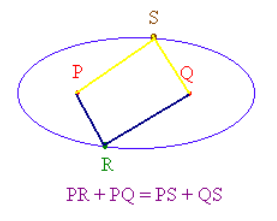
Draw an Ellipse With a String and Two Fixed Points

Geometrically an ellipse is defined as follows: Let P and Q be fixed points in the plane and let k be a positive real number. Then a point R is in the ellipse if the sum of the distances from P to R and from Q to R is k

PR + QR = k

$Graph of an ellipse with foci P and Q and points R and S. It shows PR + QR = PS + QS$

The Standard Form of an Ellipse Centered at The Origin

Recall that the equation of a circle centered at the origin has equation

x² + y² = r²

where r is the radius. Dividing by r² we have

        x²            y²
                +               =   1
        r²             r²

for an ellipse there are two radii, so that we can expect that the denominators should be different. Hence we have the standard form of an ellipse centered at the origin:

        x²            y²
                +               =   1
        a²             b²

The points (a,0), (-a,0), (0,b), and (0,-b) are called the vertices of the ellipse.

Note: Although we have written the a below the x and the b below the y, it is customary to let a be the larger of the two and b be the smaller.

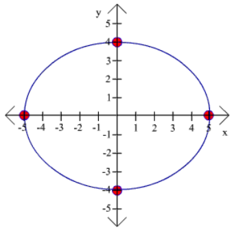
Example

Graph the ellipse

           x²               y²
                   +                 =   1
          25               16

Solution

First identify a and b, remembering to take square roots.

a = 5 b = 4

Next plot the vertices

(-5,0), (5,0), (0,4), and (0,-4)

Finally, connect the dots. The graph is shown below.

$Graph of the ellipse centered at (0,0) with x-intrecpts -5 and 5, and y-intercepts -4 and 4.$

Example

Graph the ellipse

4x² + y² = 16

Solution

This is not in standard form since the right hand side is not 1. To rectify this, we just divide by 36 to get

          4x²              y²
                   +                 =   1
          16               16

or since 9/36 = 1/4, we get

           x²               y²
                   +                 =   1
           4               16

Now we can sketch the graph. Notice that 16 is larger than 4 so we let a be the square root of 16 and b be the square root of 4. We have

a = 4 and b = 2

We plot the vertices

(0,4), (0,-4), (2,0), and (-2,0)

and connect the vertices with a conic as shown below.

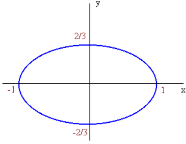
$Graph of the ellipse centered at (0,0) with x-intrecpts -2 and 2, and y-intercepts -4 and 4.$

Example

Graph the ellipse

4x² + 9y² = 4

Solution:

First divide by 4

x² + 9/4y² = 1

Since the 9/4 is not in the denominator, we need to use the following fact about division of numbers

         9                  1
                   =
         4                4/9

This comes from looking at the right hand side and and noticing that it is just a division of the fraction 1/1 by 4/9, which becomes a multiplication of 1/1 by 9/4.

        x²            y²
                +                =   1
        1             4/9

so that

a = 1 and b = 2/3

$Graph of the ellipse centered at (0,0) with x-intrecpts -1 and 1, and y-intercepts -2/3 and 2/3.$

Application: Astronomy

Suppose that an asteroid orbits the sun (in an elliptical orbit). And suppose that the longest opposite ends of the orbit are 800 million miles apart and that the shortest opposite ends are 200 million miles apart. Give an equation for the orbit of the asteroid.

Solution:

We have

2a = 800 million miles

and

2b = 200 million miles

thus

a = 400 million miles and b = 100 million miles

so that

                 x²                  y²
                                       +                                   =   1
        (400,000,000)²              (100,000,000)²

The Hyperbola

Recall the equation of the ellipse:

        x²            y²
                +               =   1
        a²             b²

If instead of a "+" we have a "-", we end up with a different conic called the hyperbola.

        x²            y²
                -               =   1
        a²             b²

Example

Sketch the graph of

        x²            y²
                -               =   1
        4              9

Solution

Check for intercepts:

If x = 0 then

              y²
          -         = 1 which has no solution
              9

If y = 0 then

           x²
                  = 1
           4

x² = 4

so that

x = 2 or x = -2

If instead of the 1, we have a 0 then

        x²            y²
                -               =   0
        4             9

so that

        x²            y²
                =
        4              9

hence

y = (3/2)x or y = -(3/2)x

These two lines are called the asymptotes of the hyperbola and are found by

y = b/a

To plot the hyperbola with equation

        x²            y²
                -               =   1
        a²             b²

we follow these steps:

Plot the intercepts

(a,0), (-a,0)

and the points

(0,b), (0,-b)

as with the ellipse.
Draw a rectangle containing these four points.
Draw the lines that contain the diagonals of the rectangle (these are the asymptotes)
Draw the hyperbola that with the vertices

(a,0) and (-a,0)

that has the drawn asymptotes.

Following these steps, to sketch the graph of

        x²            y²
                -               =   1
        4             16

We have

a = 2 and b = 4

The vertices are at

(2,0) and (-2,0)

and the helper points are at

(0,4) and (0,-4)

Plot these points. Then draw the rectangle with vertices (2,4), (-2,4), (-2,-4), and (2,-4).

Next draw the two lines through the opposite vertices of the rectangle. These are the asymptotes. Finally draw the hyperbola. On the right this process is shown.

Example:

Sketch the graph of

9x² - 4y² = 16

First we have to divide by 16 to get

          x²              y²
                    -                =   1
        16/9             4

We see that

a = 4/3 and b = 2

Note: If the equation is

        y²            x²
                -               =   1
        a²            b²

we follow the same procedure except that (0,a) and (0,-a) are the vertices instead of (b,0) and (-b,0).

Example:

        y²
                -   x²    =   1
        16

Here

b = 1 and a = 4

The intercepts are (0,4) and (0,-4) and the other two convenient points that make up the fundamental rectangle are (1,0) and (0,1). The graph is shown below

$Graph of the hyperbola y^2/16 - x^2 = 1 centered at (0,0) with y-intrecpts -4 and 4.$

Back to the Conics Home Page

Search

Text Color

Text Size

Margin Size

Font Type