

11.8: Piecewise Functions
- Page ID
- 248093

\( \newcommand{\vecs}[1]{\overset { \scriptstyle \rightharpoonup} {\mathbf{#1}} } \)
\( \newcommand{\vecd}[1]{\overset{-\!-\!\rightharpoonup}{\vphantom{a}\smash {#1}}} \)
\( \newcommand{\dsum}{\displaystyle\sum\limits} \)
\( \newcommand{\dint}{\displaystyle\int\limits} \)
\( \newcommand{\dlim}{\displaystyle\lim\limits} \)
\( \newcommand{\id}{\mathrm{id}}\) \( \newcommand{\Span}{\mathrm{span}}\)
( \newcommand{\kernel}{\mathrm{null}\,}\) \( \newcommand{\range}{\mathrm{range}\,}\)
\( \newcommand{\RealPart}{\mathrm{Re}}\) \( \newcommand{\ImaginaryPart}{\mathrm{Im}}\)
\( \newcommand{\Argument}{\mathrm{Arg}}\) \( \newcommand{\norm}[1]{\| #1 \|}\)
\( \newcommand{\inner}[2]{\langle #1, #2 \rangle}\)
\( \newcommand{\Span}{\mathrm{span}}\)
\( \newcommand{\id}{\mathrm{id}}\)
\( \newcommand{\Span}{\mathrm{span}}\)
\( \newcommand{\kernel}{\mathrm{null}\,}\)
\( \newcommand{\range}{\mathrm{range}\,}\)
\( \newcommand{\RealPart}{\mathrm{Re}}\)
\( \newcommand{\ImaginaryPart}{\mathrm{Im}}\)
\( \newcommand{\Argument}{\mathrm{Arg}}\)
\( \newcommand{\norm}[1]{\| #1 \|}\)
\( \newcommand{\inner}[2]{\langle #1, #2 \rangle}\)
\( \newcommand{\Span}{\mathrm{span}}\) \( \newcommand{\AA}{\unicode[.8,0]{x212B}}\)
\( \newcommand{\vectorA}[1]{\vec{#1}} % arrow\)
\( \newcommand{\vectorAt}[1]{\vec{\text{#1}}} % arrow\)
\( \newcommand{\vectorB}[1]{\overset { \scriptstyle \rightharpoonup} {\mathbf{#1}} } \)
\( \newcommand{\vectorC}[1]{\textbf{#1}} \)
\( \newcommand{\vectorD}[1]{\overrightarrow{#1}} \)
\( \newcommand{\vectorDt}[1]{\overrightarrow{\text{#1}}} \)
\( \newcommand{\vectE}[1]{\overset{-\!-\!\rightharpoonup}{\vphantom{a}\smash{\mathbf {#1}}}} \)
\( \newcommand{\vecs}[1]{\overset { \scriptstyle \rightharpoonup} {\mathbf{#1}} } \)
\(\newcommand{\longvect}{\overrightarrow}\)
\( \newcommand{\vecd}[1]{\overset{-\!-\!\rightharpoonup}{\vphantom{a}\smash {#1}}} \)
\(\newcommand{\ket}[1]{\left| #1 \right>}\)
\(\newcommand{\bra}[1]{\left< #1 \right|}\)
\(\newcommand{\braket}[2]{\left< #1 \vphantom{#2} \right| \left. #2 \vphantom{#1} \right>}\)
\(\newcommand{\braopket}[3]{\left< #1 \vphantom{#2}\vphantom{#3} \right| #2 \vphantom{#1}\vphantom{#3} \left| #3 \vphantom{#1}\vphantom{#2} \right>}\)
\(\newcommand{\qmvec}[1]{\mathbf{\vec{#1}}}\)
\(\newcommand{\op}[1]{\hat{\mathbf{#1}}}\)
\(\newcommand{\expect}[1]{\langle #1 \rangle}\)
\(\newcommand{\dfn}[1]{\emph{\textbf{#1}}}\)
Videos
Review: Piecewise Functions
Lecture: Graphing Piecewise Functions
Example: Graph a Non-Trivial Piecewise Function
Lecture: Find the Equation of a Piecewise Function Given the Graph
Application: Writing a Piecewise Function for Your Federal Taxes Owed
Definitions and Theorems
A single formula does not always describe a function across its entire domain. A piecewise-defined function handles this by pairing several formulas with the regions of the domain on which they apply.
A piecewise-defined function (also called a piecewise function or a function defined by cases) is a function specified by two or more sub-functions, where each sub-function applies on its own portion of the domain. The portion of the domain on which a given sub-function applies is called its subdomain.
Piecewise functions are almost always written using the following notation:\[ f ( x ) = \begin{cases}
\text{subfunction 1}, & \text{if } x \text{ is in subdomain 1} \\[6pt]
\text{subfunction 2}, & \text{if } x \text{ is in subdomain 2} \\[6pt]
\text{subfunction 3}, & \text{if } x \text{ is in subdomain 3} \\[6pt]
\vdots & \vdots \\[6pt]
\end{cases} \nonumber \]Some authors prefer to use a semicolon instead of a comma following the subfunctions. Moreover, the use of "if" following the comma is a stylistic choice, with some authors preferring to use the word "for" instead (e.g., "for \(x < 2\)). A piecewise function can also be written more succinctly by leaving out both "if" and "for," as follows:\[ f ( x ) = \begin{cases}
x^2, & x < 2 \\[6pt]
e^x, & 2 \leq x < 5 \\[6pt]
\sin(x), & x \geq 5 \\[6pt]
\end{cases} \nonumber \]A value of \(x\) at which one subdomain ends and the next begins is called a breakpoint.
A piecewise definition specifies a function on a domain \(D\) if and only if the subdomains cover \(D\) and, wherever two subdomains overlap, their sub-functions produce equal outputs. In particular, if the subdomains are pairwise disjoint and their union is \(D\), then exactly one sub-function applies to each input, so the function is well-defined.
At a breakpoint, only one subdomain may claim the input, and the inequality symbols decide which one. A subdomain written with \(\leq\) or \(\geq\) includes its endpoint, while one written with \(<\) or \(>\) excludes it. Before evaluating or graphing, confirm that the input satisfies exactly one subdomain condition.
Examples
Let \(f\) be defined by\[f(x) = \begin{cases} -x+1 & \text{if } x < 0 \\ x^2 & \text{if } 0 \leq x < 2 \\ 3 & \text{if } x \geq 2 \end{cases}\nonumber\]Evaluate \(f(-3)\), \(f(1)\), and \(f(4)\).
- Solution
-
For each input, determine which subdomain contains it, then apply the matching sub-function.
Since \(-3 < 0\), the input lies in the first subdomain, so \(f(-3) = -(-3)+1 = 4\).
Since \(0 \leq 1 < 2\), the input lies in the second subdomain, so \(f(1) = 1^2 = 1\).
Since \(4 \geq 2\), the input lies in the third subdomain, so \(f(4) = 3\).
Let \(f\) be defined by\[f(x) = \begin{cases} 2x+3 & \text{if } x \leq 1 \\ x^2-4 & \text{if } x > 1 \end{cases}\nonumber\]Evaluate \(f(1)\), \(f(0)\), and \(f(3)\).
- Solution
-
The breakpoint is \(x = 1\). Because the first subdomain is written with \(\leq\), the input \(1\) belongs to it and not to the second.
Since \(1 \leq 1\), \(f(1) = 2(1)+3 = 5\).
Since \(0 \leq 1\), \(f(0) = 2(0)+3 = 3\).
Since \(3 > 1\), \(f(3) = 3^2-4 = 5\).
Write \(f(x) = |x-3|\) as a piecewise-defined function.
- Solution
-
The absolute value of a quantity equals the quantity itself when the quantity is nonnegative, and equals its opposite when the quantity is negative. Here \(x-3 \geq 0\) exactly when \(x \geq 3\), so\[|x-3| = \begin{cases} x-3 & \text{if } x \geq 3 \\ -(x-3) & \text{if } x < 3 \end{cases}\nonumber\]Simplifying the lower sub-function gives \(-(x-3) = 3-x\), hence\[f(x) = \begin{cases} x-3 & \text{if } x \geq 3 \\ 3-x & \text{if } x < 3 \end{cases}\nonumber\]
Graph\[f(x) = \begin{cases} -x-1 & \text{if } x \leq 0 \\ 2x-1 & \text{if } x > 0 \end{cases}\nonumber\]
- Solution
-
Graph each sub-function only over its subdomain. The first piece is the line \(y = -x-1\), drawn for \(x \leq 0\); it passes through \((-2,1)\) and ends at \((0,-1)\), which is included and so drawn as a closed dot. The second piece is the line \(y = 2x-1\), drawn for \(x > 0\); it passes through \((2,3)\), and as \(x\) approaches \(0\) from the right its height approaches \(-1\). Because both pieces meet at \((0,-1)\), the graph has no break there.

Figure \(\PageIndex{1}\): The graph of \(f\).

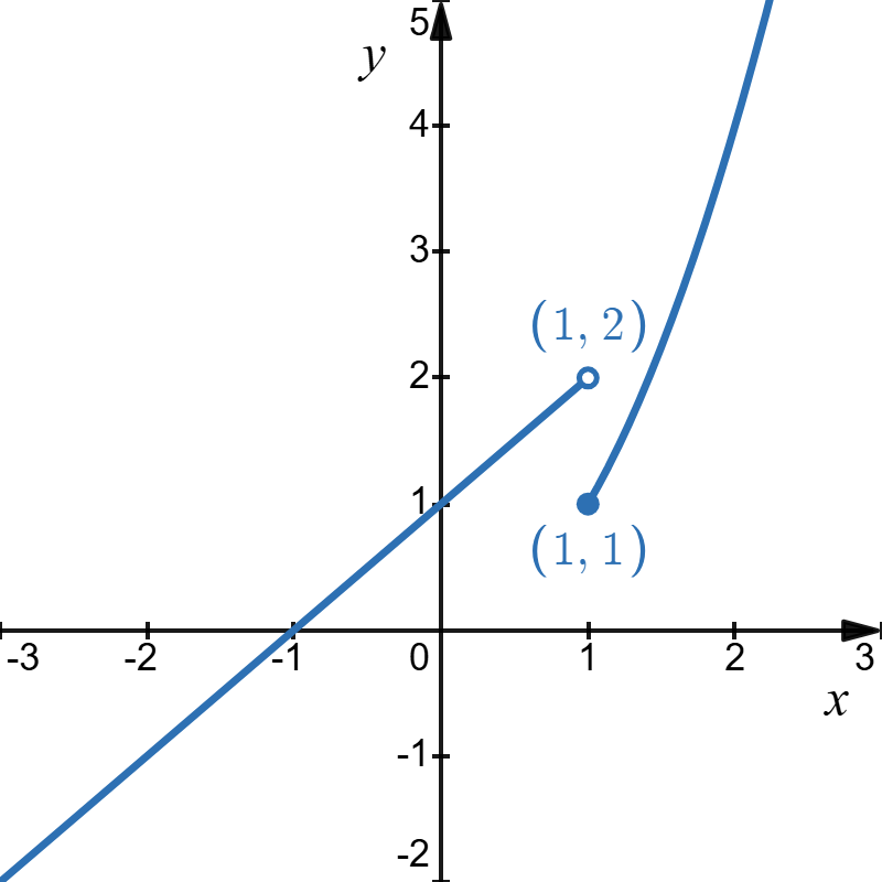
Graph\[f(x) = \begin{cases} x+1 & \text{if } x < 1 \\ x^2 & \text{if } x \geq 1 \end{cases}\nonumber\]
- Solution
-
Graph each sub-function over its subdomain. The first piece is the line \(y = x+1\), drawn for \(x < 1\); it passes through \((-1,0)\), and as \(x\) approaches \(1\) from the left its height approaches \(2\). Because \(x = 1\) is excluded from this piece, mark \((1,2)\) with an open circle. The second piece is the parabola \(y = x^2\), drawn for \(x \geq 1\); since \(x = 1\) is included, it begins at \((1,1)\) with a closed dot and passes through \((2,4)\). The left piece approaches height \(2\) while the right piece starts at height \(1\), so the graph jumps at \(x = 1\).

Figure \(\PageIndex{2}\): The graph of \(f\).
Let \(f\) be defined by\[f(x) = \begin{cases} -2 & \text{if } x < -1 \\ x+1 & \text{if } -1 \leq x \leq 2 \\ x^2 & \text{if } x > 2 \end{cases}\nonumber\]Evaluate \(f(-4)\), \(f(-1)\), \(f(2)\), and \(f(5)\), stating which sub-function applies in each case.
- Solution
-
Both breakpoints, \(-1\) and \(2\), belong to the middle subdomain, since it is written with \(\leq\) at each end.
Since \(-4 < -1\), the constant sub-function applies, so \(f(-4) = -2\).
Since \(-1 \leq -1 \leq 2\), the middle sub-function applies, so \(f(-1) = -1+1 = 0\).
Since \(-1 \leq 2 \leq 2\), the middle sub-function applies, so \(f(2) = 2+1 = 3\).
Since \(5 > 2\), the third sub-function applies, so \(f(5) = 5^2 = 25\).
MyOpenMath Practice
Sources
Several parts of this text use modifications from the following source:
- Wikipedia article: "Piecewise function"
This source is released under the Creative Commons Attribution-Share-Alike License 4.0.