11.5.4: Solving Linear Equations in One Variable

Last updated
Save as PDF

Page ID: 44671

$ \newcommand{\vecs}[1]{\overset { \scriptstyle \rightharpoonup} {\mathbf{#1}} } $

$ \newcommand{\vecd}[1]{\overset{-\!-\!\rightharpoonup}{\vphantom{a}\smash {#1}}} $

$ \newcommand{\id}{\mathrm{id}}$ $ \newcommand{\Span}{\mathrm{span}}$

( \newcommand{\kernel}{\mathrm{null}\,}\) $ \newcommand{\range}{\mathrm{range}\,}$

$ \newcommand{\RealPart}{\mathrm{Re}}$ $ \newcommand{\ImaginaryPart}{\mathrm{Im}}$

$ \newcommand{\Argument}{\mathrm{Arg}}$ $ \newcommand{\norm}[1]{\| #1 \|}$

$ \newcommand{\inner}[2]{\langle #1, #2 \rangle}$

$ \newcommand{\Span}{\mathrm{span}}$

$ \newcommand{\id}{\mathrm{id}}$

$ \newcommand{\Span}{\mathrm{span}}$

$ \newcommand{\kernel}{\mathrm{null}\,}$

$ \newcommand{\range}{\mathrm{range}\,}$

$ \newcommand{\RealPart}{\mathrm{Re}}$

$ \newcommand{\ImaginaryPart}{\mathrm{Im}}$

$ \newcommand{\Argument}{\mathrm{Arg}}$

$ \newcommand{\norm}[1]{\| #1 \|}$

$ \newcommand{\inner}[2]{\langle #1, #2 \rangle}$

$ \newcommand{\Span}{\mathrm{span}}$ $ \newcommand{\AA}{\unicode[.8,0]{x212B}}$

$ \newcommand{\vectorA}[1]{\vec{#1}} % arrow$

$ \newcommand{\vectorAt}[1]{\vec{\text{#1}}} % arrow$

$ \newcommand{\vectorB}[1]{\overset { \scriptstyle \rightharpoonup} {\mathbf{#1}} } $

$ \newcommand{\vectorC}[1]{\textbf{#1}} $

$ \newcommand{\vectorD}[1]{\overrightarrow{#1}} $

$ \newcommand{\vectorDt}[1]{\overrightarrow{\text{#1}}} $

$ \newcommand{\vectE}[1]{\overset{-\!-\!\rightharpoonup}{\vphantom{a}\smash{\mathbf {#1}}}} $

$ \newcommand{\vecs}[1]{\overset { \scriptstyle \rightharpoonup} {\mathbf{#1}} } $

$ \newcommand{\vecd}[1]{\overset{-\!-\!\rightharpoonup}{\vphantom{a}\smash {#1}}} $

$\newcommand{\avec}{\mathbf a}$ $\newcommand{\bvec}{\mathbf b}$ $\newcommand{\cvec}{\mathbf c}$ $\newcommand{\dvec}{\mathbf d}$ $\newcommand{\dtil}{\widetilde{\mathbf d}}$ $\newcommand{\evec}{\mathbf e}$ $\newcommand{\fvec}{\mathbf f}$ $\newcommand{\nvec}{\mathbf n}$ $\newcommand{\pvec}{\mathbf p}$ $\newcommand{\qvec}{\mathbf q}$ $\newcommand{\svec}{\mathbf s}$ $\newcommand{\tvec}{\mathbf t}$ $\newcommand{\uvec}{\mathbf u}$ $\newcommand{\vvec}{\mathbf v}$ $\newcommand{\wvec}{\mathbf w}$ $\newcommand{\xvec}{\mathbf x}$ $\newcommand{\yvec}{\mathbf y}$ $\newcommand{\zvec}{\mathbf z}$ $\newcommand{\rvec}{\mathbf r}$ $\newcommand{\mvec}{\mathbf m}$ $\newcommand{\zerovec}{\mathbf 0}$ $\newcommand{\onevec}{\mathbf 1}$ $\newcommand{\real}{\mathbb R}$ $\newcommand{\twovec}[2]{\left[\begin{array}{r}#1 \\ #2 \end{array}\right]}$ $\newcommand{\ctwovec}[2]{\left[\begin{array}{c}#1 \\ #2 \end{array}\right]}$ $\newcommand{\threevec}[3]{\left[\begin{array}{r}#1 \\ #2 \\ #3 \end{array}\right]}$ $\newcommand{\cthreevec}[3]{\left[\begin{array}{c}#1 \\ #2 \\ #3 \end{array}\right]}$ $\newcommand{\fourvec}[4]{\left[\begin{array}{r}#1 \\ #2 \\ #3 \\ #4 \end{array}\right]}$ $\newcommand{\cfourvec}[4]{\left[\begin{array}{c}#1 \\ #2 \\ #3 \\ #4 \end{array}\right]}$ $\newcommand{\fivevec}[5]{\left[\begin{array}{r}#1 \\ #2 \\ #3 \\ #4 \\ #5 \\ \end{array}\right]}$ $\newcommand{\cfivevec}[5]{\left[\begin{array}{c}#1 \\ #2 \\ #3 \\ #4 \\ #5 \\ \end{array}\right]}$ $\newcommand{\mattwo}[4]{\left[\begin{array}{rr}#1 \amp #2 \\ #3 \amp #4 \\ \end{array}\right]}$ $\newcommand{\laspan}[1]{\text{Span}\{#1\}}$ $\newcommand{\bcal}{\cal B}$ $\newcommand{\ccal}{\cal C}$ $\newcommand{\scal}{\cal S}$ $\newcommand{\wcal}{\cal W}$ $\newcommand{\ecal}{\cal E}$ $\newcommand{\coords}[2]{\left\{#1\right\}_{#2}}$ $\newcommand{\gray}[1]{\color{gray}{#1}}$ $\newcommand{\lgray}[1]{\color{lightgray}{#1}}$ $\newcommand{\rank}{\operatorname{rank}}$ $\newcommand{\row}{\text{Row}}$ $\newcommand{\col}{\text{Col}}$ $\renewcommand{\row}{\text{Row}}$ $\newcommand{\nul}{\text{Nul}}$ $\newcommand{\var}{\text{Var}}$ $\newcommand{\corr}{\text{corr}}$ $\newcommand{\len}[1]{\left|#1\right|}$ $\newcommand{\bbar}{\overline{\bvec}}$ $\newcommand{\bhat}{\widehat{\bvec}}$ $\newcommand{\bperp}{\bvec^\perp}$ $\newcommand{\xhat}{\widehat{\xvec}}$ $\newcommand{\vhat}{\widehat{\vvec}}$ $\newcommand{\uhat}{\widehat{\uvec}}$ $\newcommand{\what}{\widehat{\wvec}}$ $\newcommand{\Sighat}{\widehat{\Sigma}}$ $\newcommand{\lt}{<}$ $\newcommand{\gt}{>}$ $\newcommand{\amp}{&}$ $\definecolor{fillinmathshade}{gray}{0.9}$

Learning Outcomes

Solve linear equations for the variable.

It is a common task in algebra to solve an equation for a variable. The goal will be to get the variable on one side of the equation all by itself and have the other side of the equation just be a number. The process will involve identifying the operations that are done on the variable and apply the inverse operation to both sides of the equation. This will be managed in the reverse of the order of operations.

Example $\PageIndex{1}$

Solve the following equation for $x$.

\[3x+4=11 \label{EQ1.1}\]

Solution

We begin by looking at the operations that are done to $x$, keeping track the order. The first operation is "multiply by 3" and the second is "add 4". We now do everything backwards. Since the last operation is "add 4", our first step is to subtract 4 from both sides of Equation \ref{EQ1.1}.

\[3x \cancel{+ 4} \color{Cerulean}{ \cancel{-4}} \color{black} =11 \color{Cerulean}{ -4} \nonumber\]

which simplifies the equation

\[3x = 7 \nonumber\]

Next, the way to undo "multiply by 3" is to divide both sides by 3. We get

\[ \dfrac{\cancel{3}x}{\color{Cerulean}{\cancel{3}}} \color{black}= \dfrac{7}{\color{Cerulean}{3}} \nonumber\]

\[x=\dfrac{7}{3} \nonumber\]

Example $\PageIndex{2}$

The rectangle above is a diagram for a uniform distribution from 2 to 9 that asks for the first quartile. The area of the smaller red rectangle that has base from 2 to Q1 and height 1/7 is 1/4. Find Q1.

Solution

We start by using the area formula for a rectangle:

\[\text{Area} = \text{Base} \times \text{Height} \label{EQ1}\]

We have:

Area = $\frac{1}{4}$
Base = $Q1-2$
Height = $\frac{1}{7}$

Plug this into Equation \ref{EQ1} to get:

\[\frac{1}{4}=\left(Q1-2\right)\left(\frac{1}{7}\right) \label{EQ2}\]

We need to solve for $Q1$. First multiple both sides of Equation \ref{EQ2} by 7 to get:

\[ \begin{align} \color{Cerulean}{7} \color{black} \left(\dfrac{1}{4}\right) &= \color{Cerulean}{\cancel{7}} \color{black} \left(Q1-2\right) \cancel{ \left(\frac{1}{7}\right)} \nonumber \\[5pt] \dfrac{7}{4} &=Q1-2 \label{EQ4} \end{align}\]

Now add 2 to both sides of Equation \ref{EQ4} to get:

\[ \begin{align*} \dfrac{7}{4} \color{Cerulean} +2 \color{black} & =Q1 \cancel{-2} \color{Cerulean}{\cancel{+2}} \\[5pt] \dfrac{7}{4}+2&=Q1 \end{align*}\]

\[Q1=\frac{7}{4}+2 \nonumber\]

Putting this into a calculator gives:

\[Q1=3.75 \nonumber\]

Example $\PageIndex{3}$: z-score

The z-score for a given value $x$ for a distribution with population mean $\mu $ and population standard deviation $\sigma $ is given by:

\[z=\frac{x-\mu}{\sigma} \nonumber\]

An online retailer has found that the population mean sales per day is $2,841 and the population standard deviation is $895. A value of $x$ is considered an outlier if the z-score is less than -2 or greater than 2. How many sales must be made to have a z-score of 2?

Solution

First we identify each of the given variables. Since the population mean is 2,841, we have:

\[\mu=2841 \nonumber \]

We are told that the population standard deviation is 895 meters, so:

\[\sigma=895 \nonumber \]

We are also given that the z-score is 2, hence:

\[z=2 \nonumber \]

Now we put the numbers into the formula for the z-score to get:

\[2=\frac{x-2841}{895} \nonumber \]

We can next switch the order of the equation so that the $x$ is on the left hand side of the equation:

\[\frac{x-2841}{895}=2 \nonumber \]

Next, we solve for $x$. First multiply both sides of the equation by 895 to get

\[x-2841=2\left(895\right)=1790 \nonumber \]

Finally, we can add 2841 to both sides of the equation to get $x$ by itself:

\[x=1790+2841=4631 \nonumber \]

We can conclude that if the day's sales is at $4631, the z-score is 2.

Exercise

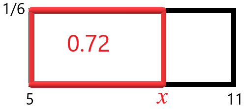
The rectangle below is a diagram for a uniform distribution from 5 to 11 that asks for the 72^nd percentile. The area of the smaller red rectangle that has base from 5 to the 72^nd percentile, $x$, and height 1/6 is 0.72. Find $x$.

rectangle: outer base 5 to 11, inner base 5 to x, height 1/6

Search

Text Color

Text Size

Margin Size

Font Type