14.2: Measures of Central Tendency

Last updated
Save as PDF

Page ID: 96495

David Lippman & Jeff Eldridge
Pierce College via The OpenTextBookStore

$ \newcommand{\vecs}[1]{\overset { \scriptstyle \rightharpoonup} {\mathbf{#1}} } $ $ \newcommand{\vecd}[1]{\overset{-\!-\!\rightharpoonup}{\vphantom{a}\smash {#1}}} $$\newcommand{\id}{\mathrm{id}}$ $ \newcommand{\Span}{\mathrm{span}}$ $ \newcommand{\kernel}{\mathrm{null}\,}$ $ \newcommand{\range}{\mathrm{range}\,}$ $ \newcommand{\RealPart}{\mathrm{Re}}$ $ \newcommand{\ImaginaryPart}{\mathrm{Im}}$ $ \newcommand{\Argument}{\mathrm{Arg}}$ $ \newcommand{\norm}[1]{\| #1 \|}$ $ \newcommand{\inner}[2]{\langle #1, #2 \rangle}$ $ \newcommand{\Span}{\mathrm{span}}$ $\newcommand{\id}{\mathrm{id}}$ $ \newcommand{\Span}{\mathrm{span}}$ $ \newcommand{\kernel}{\mathrm{null}\,}$ $ \newcommand{\range}{\mathrm{range}\,}$ $ \newcommand{\RealPart}{\mathrm{Re}}$ $ \newcommand{\ImaginaryPart}{\mathrm{Im}}$ $ \newcommand{\Argument}{\mathrm{Arg}}$ $ \newcommand{\norm}[1]{\| #1 \|}$ $ \newcommand{\inner}[2]{\langle #1, #2 \rangle}$ $ \newcommand{\Span}{\mathrm{span}}$$\newcommand{\AA}{\unicode[.8,0]{x212B}}$

Let's begin by trying to find the most "typical" value of a data set.

Note that we just used the word "typical" although in many cases you might think of using the word "average." We need to be careful with the word "average" as it means different things to different people in different contexts. One of the most common uses of the word "average" is what mathematicians and statisticians call the arithmetic mean, or just plain old mean for short. "Arithmetic mean" sounds rather fancy, but you have likely calculated a mean many times without realizing it; the mean is what most people think of when they use the word "average".

Mean

The mean of a set of data is the sum of the data values divided by the number of values.

Example 1

Marci’s exam scores for her last math class were: 79, 86, 82, 94. The mean of these values would be:

Solution

\[\frac{79+86+82+94}{4}=85.25. \nonumber\]

Typically we round means to one more decimal place than the original data had. In this case, we would round 85.25 to 85.3.

Example 2

The number of touchdown (TD) passes thrown by each of the 31 teams in the National Football League in the 2000 season are shown below.

37 33 33 32 29 28 28 23 22 22 22 21 21 21 20

20 19 19 18 18 18 18 16 15 14 14 14 12 12 9 6

Solution

Adding these values, we get 634 total TDs. Dividing by 31, the number of data values, we get $\frac{634}{31} = 20.4516$. It would be appropriate to round this to 20.5.

It would be most correct for us to report that “The mean number of touchdown passes thrown in the NFL in the 2000 season was 20.5 passes,” but it is not uncommon to see the more casual word “average” used in place of “mean.

Try it Now 1

The price of a jar of peanut butter at 5 stores was: $3.29, $3.59, $3.79, $3.75, and $3.99. Find the mean price.

Answer: The mean price is $3.68

Example 3

The one hundred families in a particular neighborhood are asked their annual household income, to the nearest $5 thousand dollars. The results are summarized in a frequency table below.

$\begin{array}{|l|l|}
\hline \textbf { Income (thousands of dollars) } & \textbf { Frequency } \\
\hline 15 & 6 \\
\hline 20 & 8 \\
\hline 25 & 11 \\
\hline 30 & 17 \\
\hline 35 & 19 \\
\hline 40 & 20 \\
\hline 45 & 12 \\
\hline 50 & 7 \\
\hline
\end{array}$

Solution

Calculating the mean by hand could get tricky if we try to type in all 100 values:

\[\frac{15 + \cdots + 15 + 20 + \cdots+20 + 25 + \cdots + 25 + \cdots}{100} \nonumber\]

We could calculate this more easily by noticing that adding 15 to itself six times is the same as $15 \cdot 6=90$. Using this simplification, we get

\[\frac{15 \cdot 6+20 \cdot 8+25 \cdot 11+30 \cdot 17+35 \cdot 19+40 \cdot 20+45 \cdot 12+50 \cdot 7}{100}=\frac{3390}{100}=33.9 \nonumber\]

The mean household income of our sample is 33.9 thousand dollars ($33,900).

Example 4

Extending off the last example, suppose a new family moves into the neighborhood example that has a household income of $5 million ($5000 thousand). Adding this to our sample, our mean is now:

Solution

\[\frac{15 \cdot 6+20 \cdot 8+25 \cdot 11+30 \cdot 17+35 \cdot 19+40 \cdot 20+45 \cdot 12+50 \cdot 7+5000 \cdot 1}{101}=\frac{8390}{101}=83.069 \nonumber\]

While 83.1 thousand dollars ($83,069) is the correct mean household income, it no longer represents a “typical” value.

Imagine the data values on a see-saw or balance scale. The mean is the value that keeps the data in balance, like in the picture below.

$dd21.svg$

If we graph our household data, the $5 million data value is so far out to the right that the mean has to adjust up to keep things in balance

$dd22.svg$

For this reason, when working with data that have outliers – values far outside the primary grouping – it is common to use a different measure of center, the median.

Median

To find the median, begin by listing the data in order from smallest to largest.

If the number of data values, $N$, is odd, then the median is the middle data value. This value can be found by rounding $\frac{N}{2}$ up to the next whole number.

If the number of data values is even, there is no one middle value, so we find the mean of the two middle values (values $\frac{N}{2}$ and $\frac{N}{2} + 1$)

Example 5

Returning to the football touchdown data, we would start by listing the data in order. We need to put the data in order from smallest to largest.

6 9 12 12 14 14 14 15 16 18 18 18 18 19 19 20 20 21 21 21 22 22 22 23 28 28 29 32 33 33 37

Solution

Since there are 31 data values, an odd number, the median will be the middle number, the 16^th data value (\frac{31}{2} = 15.5\), round up to 16, leaving 15 values below and 15 above). The 16^th data value is 20, so the median number of touchdown passes in the 2000 season was 20 passes. Notice that for this data, the median is fairly close to the mean we calculated earlier, 20.5.

Example 6

Find the median of these quiz scores: 5 10 8 6 4 8 2 5 7 7

We start by listing the data in order: 2 4 5 5 6 7 7 8 8 10

Solution

Since there are 10 data values, an even number, there is no one middle number. So we find the mean of the two middle numbers, 6 and 7, and get $\frac{6+7}{2} = 6.5$.

The median quiz score was 6.5.

Try it Now 2

The price of a jar of peanut butter at 5 stores were: $3.29, $3.59, $3.79, $3.75, and $3.99. Find the median price.

Answer: First we put the data in order: $3.29, $3.59, $3.75, $3.79, $3.99. Since there are an odd number of data, the median will be the middle value, $3.75.

Example 7

Let us return now to our original household income data

Solution

Here we have 100 data values. If we didn’t already know that, we could find it by adding the frequencies. Since 100 is an even number, we need to find the mean of the middle two data values - the 50^th and 51^st data values. To find these, we start counting up from the bottom:

\[\begin{array}{ll} \text{There are 6 data values of \$15, so} & \text{Values 1 to } 6 \text{ are \$15 thousand } \\ \text{The next 8 data values are \$20, so } & \text{Values 7 to } (6+8)=14 \text{ are \$20 thousand} \\ \text{The next 11 data values are \$25, so} & \text{ Values 15 to } (14+11)=25 \text{ are \$25 thousand} \\ \text{The next 17 data values are \$30, so} & \text{Values 26 to } (25+17)=42 \text{ are \$30 thousand} \\ \text{The next 19 data values are \$35, so} & \text{Values 43 to } (42+19)=61 \text{ are \$35 thousand} \end{array}\]

From this we can tell that values 50 and 51 will be $35 thousand, and the mean of these two values is $35 thousand. The median income in this neighborhood is $35 thousand.

Example 8

If we add in the new neighbor with a $5 million household income, then there will be 101 data values, and the 51^st value will be the median. As we discovered in the last example, the 51^st value is $35 thousand. Notice that the new neighbor did not affect the median in this case. The median is not swayed as much by outliers as the mean is.

In addition to the mean and the median, there is one other common measurement of the "typical" value of a data set: the mode.

Mode

The mode is the element(s) of the data set that occurs most frequently. It is possible for a data set to have more than one mode if several categories have the same frequency, or no modes if each every category occurs only once.

The mode is fairly useless with data like weights or heights where there are a large number of possible values. The mode is most commonly used for categorical data, for which median and mean cannot be computed.

Example 9

In our vehicle color survey, we collected the data

$\begin{array}{|l|l|}
\hline \textbf { Color } & \textbf { Frequency } \\
\hline \text { Blue } & 3 \\
\hline \text { Green } & 5 \\
\hline \text { Red } & 4 \\
\hline \text { White } & 3 \\
\hline \text { Black } & 2 \\
\hline \text { Grey } & 3 \\
\hline
\end{array}$

For this data, Green is the mode, since it is the data value that occurred the most frequently.

Example 10

Look back to the quiz scores example: 2 4 5 5 6 7 7 8 8 10. Find the mode of this data set.

Solution

Since 5, 7, and 8 all occur twice and that is more than any other value in the set, we say that 5, 7, and 8 are all modes.

Example 11

Marci’s exam scores for her last math class were: 79, 86, 82, 94. Find the mode of this data set.

Solution

Since none of the values are ever repeated, this data set has no mode.

Try it Now 3

Reviewers were asked to rate a product on a scale of 1 to 5. Find

The mean rating
The median rating
The mode rating

$\begin{array}{|l|l|}
\hline \textbf { Rating } & \textbf { Frequency } \\
\hline 1 & 4 \\
\hline 2 & 8 \\
\hline 3 & 7 \\
\hline 4 & 3 \\
\hline 5 & 1 \\
\hline
\end{array}$

Answer

The mean is $\frac{1 \cdot 4+2 \cdot 8+3 \cdot 7+4 \cdot 3+5 \cdot 1}{23} \approx 2.5$
There are 23 data values, so the median will be the 12^th data value. Ratings of 1 are the first 4 values, while a rating of 2 are the next 8 values, so the 12^th value will be a rating of 2. The median is 2.
The mode is the most frequent rating. The mode rating is 2.

Quartiles

Quartiles are values that divide the data in quarters.

The first quartile ($Q_1$) is the value so that 25% of the data values are below it; the third quartile ($Q_3$) is the value so that 75% of the data values are below it. You may have guessed that the second quartile is the same as the median, since the median is the value so that 50% of the data values are below it.

This divides the data into quarters; 25% of the data is between the minimum and $Q_1$, 25% is between $Q_1$ and the median, 25% is between the median and $Q_3$, and 25% is between $Q_3$ and the maximum value

To Find Quartiles

To find the quartiles of a data set:
Step 1: Sort the data set from the smallest value to the largest value.
Step 2: Find the median (Q2). This cuts the data into two halves.
Step 3: Find the median of the lower 50% of the data values. This is the first quartile (Q1).
Step 4: Find the median of the upper 50% of the data values. This is the third quartile (Q3).

Examples should help make this clearer.

Example 12

Suppose we have measured 9 females and their heights (in inches), sorted from smallest to largest are:

59 60 62 64 66 67 69 70 72

Since the number of values is odd, the median (Q2) is the middle number 66.

To find the first quartile, we find the median of the lower half: 59 60 62 64. So Q1 = $\frac{60+62}{2}$ = 61.

To find the third quartile, we find the median of the upper half: 67 69 70 72. So Q3 = $\frac{69+70}{2}$ = 69.5

Example 13

Suppose we had measured 8 females and their heights (in inches), sorted from smallest to largest are:

59 60 62 64 66 67 69 70

Since there are an even number of data values, the median is $\frac{64+66}{2}$ = 65

To find the first quartile, we find the median of the bottom half: 59 60 62 64. So Q1 = $\frac{60+62}{2}$ = 61.

The find the third quartile, we find the median of the top half: 66 67 69 70. So Q3 = $\frac{67+69}{2}$ = 68

The 5-number summary combines the first and third quartile with the minimum, median, and maximum values.

Five Number Summary

The five number summary takes this form:

Minimum, $Q_1$, Median, $Q_3$, Maximum

Example 14

For the 9 female sample, the minimum is 59, and the maximum is 72. The 5 number summary is: 59, 61, 66, 69.5, 72.

For the 8 female sample, the minimum is 59, and the maximum is 70, so the 5 number summary would be: 59, 61, 65, 68, 70.

Try it Now 4

The total cost of textbooks for the term was collected from 36 students. Find the 5 number summary of this data.

$140 $160 $160 $165 $180 $220 $235 $240 $250 $260 $280 $285

$285 $285 $290 $300 $300 $305 $310 $310 $315 $315 $320 $320

$330 $340 $345 $350 $355 $360 $360 $380 $395 $420 $460 $460

Answer

The data is already in order, so we don’t need to sort it first.

The minimum value is $140 and the maximum is $460.

There are 36 data values so $n=36 . n / 2=18,$ which is a whole number, so the median is the mean of the $18^{\text {th }}$ and $19^{\text {th }}$ data values, $\$ 305$ and $\$ 310$. The median is $\$ 307.50$

To find the first quartile, we find the median of the lower half:

$140 $160 $160 $165 $180 $220 $235 $240 $250 $260 $280 $285 $285 $285 $290 $300 $300 $305

Q1 = $\frac{$250+$260}{2}$ = $255

To find the third quartile, we find the median of the upper half:

$310 $310 $315 $315 $320 $320 $330 $340 $345 $350 $355 $360 $360 $380 $395 $420 $460 $460

Q3 = $\frac{$345+$350}{2}$ = $347.50

The 5 number summary of this data is: $140, $255, $307.50, $347.50, $460

Also, since we have the quartiles, we can talk about how much spread there is between the 1st and 3rd quartiles. This is known as the interquartile range.

Interquartile Range

The Interquartile Range of (IQR) = $Q_3$ - $Q_1$

For visualizing data, there is a graphical representation of a 5-number summary called a box plot, or box and whisker graph.

Boxplot

A box plot is a graphical representation of a five-number summary.

A box plot is created by first setting a scale (number line) as a guideline for the box plot. Then, draw a rectangle that spans from Q1 to Q3 above the number line. Mark the median with a vertical line through the rectangle. Next, draw dots for the minimum and maximum points to the sides of the rectangle. Finally, draw lines from the sides of the rectangle out to the dots.

Example 15

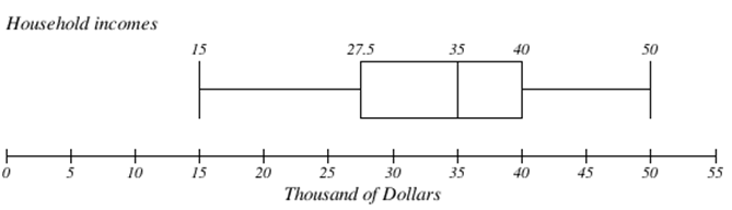
The box plot below is based on the household income data with 5 number summary:

15, 27.5, 35, 40, 50

$clipboard_eca8ff39b07909efcfda7c0322250c2e1.png$

Box plots are particularly useful for comparing data from two populations.

Example 16

The box plot of service times for two fast-food restaurants is shown below.

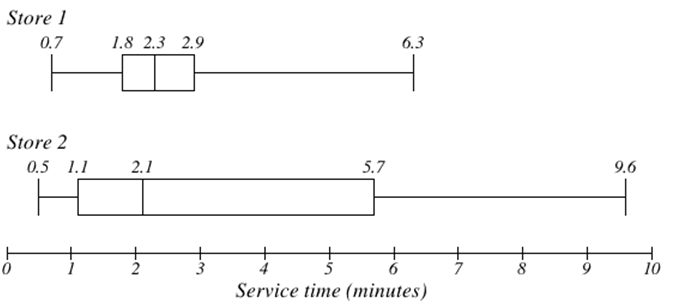
$clipboard_e293f61320982561d3363676380e95aae.png$

While store 2 had a slightly shorter median service time (2.1 minutes vs. 2.3 minutes), store 2 is less consistent, with a wider spread of the data.

At store 1, 75% of customers were served within 2.9 minutes, while at store 2, 75% of customers were served within 5.7 minutes.

Which store should you go to in a hurry? That depends upon your opinions about luck – 25% of customers at store 2 had to wait between 5.7 and 9.6 minutes.