
4.3: Probability Rules
- Page ID
- 202285

\( \newcommand{\vecs}[1]{\overset { \scriptstyle \rightharpoonup} {\mathbf{#1}} } \)
\( \newcommand{\vecd}[1]{\overset{-\!-\!\rightharpoonup}{\vphantom{a}\smash {#1}}} \)
\( \newcommand{\dsum}{\displaystyle\sum\limits} \)
\( \newcommand{\dint}{\displaystyle\int\limits} \)
\( \newcommand{\dlim}{\displaystyle\lim\limits} \)
\( \newcommand{\id}{\mathrm{id}}\) \( \newcommand{\Span}{\mathrm{span}}\)
( \newcommand{\kernel}{\mathrm{null}\,}\) \( \newcommand{\range}{\mathrm{range}\,}\)
\( \newcommand{\RealPart}{\mathrm{Re}}\) \( \newcommand{\ImaginaryPart}{\mathrm{Im}}\)
\( \newcommand{\Argument}{\mathrm{Arg}}\) \( \newcommand{\norm}[1]{\| #1 \|}\)
\( \newcommand{\inner}[2]{\langle #1, #2 \rangle}\)
\( \newcommand{\Span}{\mathrm{span}}\)
\( \newcommand{\id}{\mathrm{id}}\)
\( \newcommand{\Span}{\mathrm{span}}\)
\( \newcommand{\kernel}{\mathrm{null}\,}\)
\( \newcommand{\range}{\mathrm{range}\,}\)
\( \newcommand{\RealPart}{\mathrm{Re}}\)
\( \newcommand{\ImaginaryPart}{\mathrm{Im}}\)
\( \newcommand{\Argument}{\mathrm{Arg}}\)
\( \newcommand{\norm}[1]{\| #1 \|}\)
\( \newcommand{\inner}[2]{\langle #1, #2 \rangle}\)
\( \newcommand{\Span}{\mathrm{span}}\) \( \newcommand{\AA}{\unicode[.8,0]{x212B}}\)
\( \newcommand{\vectorA}[1]{\vec{#1}} % arrow\)
\( \newcommand{\vectorAt}[1]{\vec{\text{#1}}} % arrow\)
\( \newcommand{\vectorB}[1]{\overset { \scriptstyle \rightharpoonup} {\mathbf{#1}} } \)
\( \newcommand{\vectorC}[1]{\textbf{#1}} \)
\( \newcommand{\vectorD}[1]{\overrightarrow{#1}} \)
\( \newcommand{\vectorDt}[1]{\overrightarrow{\text{#1}}} \)
\( \newcommand{\vectE}[1]{\overset{-\!-\!\rightharpoonup}{\vphantom{a}\smash{\mathbf {#1}}}} \)
\( \newcommand{\vecs}[1]{\overset { \scriptstyle \rightharpoonup} {\mathbf{#1}} } \)
\(\newcommand{\longvect}{\overrightarrow}\)
\( \newcommand{\vecd}[1]{\overset{-\!-\!\rightharpoonup}{\vphantom{a}\smash {#1}}} \)
\(\newcommand{\avec}{\mathbf a}\) \(\newcommand{\bvec}{\mathbf b}\) \(\newcommand{\cvec}{\mathbf c}\) \(\newcommand{\dvec}{\mathbf d}\) \(\newcommand{\dtil}{\widetilde{\mathbf d}}\) \(\newcommand{\evec}{\mathbf e}\) \(\newcommand{\fvec}{\mathbf f}\) \(\newcommand{\nvec}{\mathbf n}\) \(\newcommand{\pvec}{\mathbf p}\) \(\newcommand{\qvec}{\mathbf q}\) \(\newcommand{\svec}{\mathbf s}\) \(\newcommand{\tvec}{\mathbf t}\) \(\newcommand{\uvec}{\mathbf u}\) \(\newcommand{\vvec}{\mathbf v}\) \(\newcommand{\wvec}{\mathbf w}\) \(\newcommand{\xvec}{\mathbf x}\) \(\newcommand{\yvec}{\mathbf y}\) \(\newcommand{\zvec}{\mathbf z}\) \(\newcommand{\rvec}{\mathbf r}\) \(\newcommand{\mvec}{\mathbf m}\) \(\newcommand{\zerovec}{\mathbf 0}\) \(\newcommand{\onevec}{\mathbf 1}\) \(\newcommand{\real}{\mathbb R}\) \(\newcommand{\twovec}[2]{\left[\begin{array}{r}#1 \\ #2 \end{array}\right]}\) \(\newcommand{\ctwovec}[2]{\left[\begin{array}{c}#1 \\ #2 \end{array}\right]}\) \(\newcommand{\threevec}[3]{\left[\begin{array}{r}#1 \\ #2 \\ #3 \end{array}\right]}\) \(\newcommand{\cthreevec}[3]{\left[\begin{array}{c}#1 \\ #2 \\ #3 \end{array}\right]}\) \(\newcommand{\fourvec}[4]{\left[\begin{array}{r}#1 \\ #2 \\ #3 \\ #4 \end{array}\right]}\) \(\newcommand{\cfourvec}[4]{\left[\begin{array}{c}#1 \\ #2 \\ #3 \\ #4 \end{array}\right]}\) \(\newcommand{\fivevec}[5]{\left[\begin{array}{r}#1 \\ #2 \\ #3 \\ #4 \\ #5 \\ \end{array}\right]}\) \(\newcommand{\cfivevec}[5]{\left[\begin{array}{c}#1 \\ #2 \\ #3 \\ #4 \\ #5 \\ \end{array}\right]}\) \(\newcommand{\mattwo}[4]{\left[\begin{array}{rr}#1 \amp #2 \\ #3 \amp #4 \\ \end{array}\right]}\) \(\newcommand{\laspan}[1]{\text{Span}\{#1\}}\) \(\newcommand{\bcal}{\cal B}\) \(\newcommand{\ccal}{\cal C}\) \(\newcommand{\scal}{\cal S}\) \(\newcommand{\wcal}{\cal W}\) \(\newcommand{\ecal}{\cal E}\) \(\newcommand{\coords}[2]{\left\{#1\right\}_{#2}}\) \(\newcommand{\gray}[1]{\color{gray}{#1}}\) \(\newcommand{\lgray}[1]{\color{lightgray}{#1}}\) \(\newcommand{\rank}{\operatorname{rank}}\) \(\newcommand{\row}{\text{Row}}\) \(\newcommand{\col}{\text{Col}}\) \(\renewcommand{\row}{\text{Row}}\) \(\newcommand{\nul}{\text{Nul}}\) \(\newcommand{\var}{\text{Var}}\) \(\newcommand{\corr}{\text{corr}}\) \(\newcommand{\len}[1]{\left|#1\right|}\) \(\newcommand{\bbar}{\overline{\bvec}}\) \(\newcommand{\bhat}{\widehat{\bvec}}\) \(\newcommand{\bperp}{\bvec^\perp}\) \(\newcommand{\xhat}{\widehat{\xvec}}\) \(\newcommand{\vhat}{\widehat{\vvec}}\) \(\newcommand{\uhat}{\widehat{\uvec}}\) \(\newcommand{\what}{\widehat{\wvec}}\) \(\newcommand{\Sighat}{\widehat{\Sigma}}\) \(\newcommand{\lt}{<}\) \(\newcommand{\gt}{>}\) \(\newcommand{\amp}{&}\) \(\definecolor{fillinmathshade}{gray}{0.9}\)Section 1: Compound Events
Next, we will introduce the ways to create new events from existing ones. First, let's discuss a way to create a new event from just a single event.
Let \(E\) be an event then a new event, called the complement of \(E\), can be formed from all the outcomes that are not in \(E\). The complement of \(E\) can be labeled in many ways:
\(\text{not }E\) or \(E^c\) or \(E'\) or \(\bar{E}\)
Visually we can identify the complement of \(E\) by writing out the sample space and collecting all the outcomes that are not in \(E\).
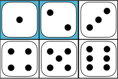
Consider the experiment of rolling a fair die with the well-known sample space:
\(\{1, 2, 3, 4, 5, 6\}\)
Consider the following events \(A\), \(B\), and \(C\) defined by the following sets:
\(A=\{1, 5\}\)
\(B=\{2, 4, 5\}\)
\(C=\{2, 3, 4, 6\}\)
Then using the definition of a complement we can find the complements of \(A\), \(B\), and \(C\):
\((\text{not }A)=\{2, 3, 4, 6\}\)
\((\text{not }B)=\{1, 3, 6\}\)
\((\text{not }C)=\{1, 5\}\)
Next, we will discuss ways to create a new event from a pair of events.
Let \(A\) and \(B\) be two events then a new event, called the intersection of A and B, can be formed from all the outcomes that are in both \(A\) and \(B\). The intersection of \(A\) and \(B\) can be labeled in a few different ways:
\((A\text{ and }B)\) or \((A \cap B)\)
Visually we can identify the intersection of \(A\) and \(B\) by writing out the sample space labeling \(A\) and \(B\) and collecting all the outcomes that are in both \(A\) and \(B\).
Using the definition of an intersection we can find the intersections \((A\text{ and }B)\), \((B\text{ and }C)\), and \((C\text{ and }A)\):
\((A\text{ and }B)=\{5\}\)
\((B\text{ and }C)=\{2, 4\}\)
\((C\text{ and }A)=\{\text{ }\}\)
Here is another way to create a new event from a pair of events.
Let \(A\) and \(B\) be two events then a new event, called the union of A and B, can be formed from all the outcomes that are in \(A\), in \(B\), and in both \(A\) and \(B\). The union of \(A\) and \(B\) can be labeled in a few different ways:
\((A\text{ or }B)\) or \((A \cup B)\)
Visually we can identify the union of \(A\) and \(B\) by writing out the sample space labeling \(A\) and \(B\) and collecting all the outcomes that are in \(A\), \(B\), or both.
Using the definition of a union we can find the unions \((A\text{ or }B)\), \((B\text{ or }C)\), and \((C\text{ or }A)\):
\((A\text{ or }B)=\{1, 2, 4, 5\}\)
\((B\text{ or }C)=\{2, 3, 4, 5, 6\}\)
\((C\text{ or }A)=\{1, 2, 3, 4, 5, 6\}\)
We introduced and discussed the idea of creating new events from an existing one or two events.
Section 2: Venn Diagrams
We can visualize events by first drawing all possible outcomes, and then circling the ones that are in the set description of the event. Such picture is called a Venn diagram. Any shape drawn on the sample space will define some event.
Each Venn diagram has the following properties:
- the box represents the sample space.
- the area of the region is \(P(E)\).
- the area of the box is 1.
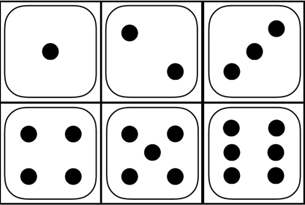
Example: This is what the Venn diagram of the sample space for rolling a die look like.
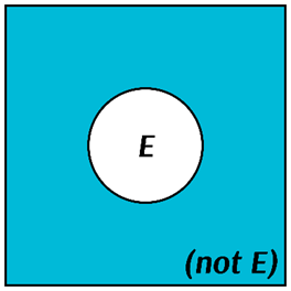
Just like the compound events are derived from events, the Venn diagrams of compound events can be derived from the Venn diagram(s) of the original event or events. For example, this is what the Venn diagram for the complement of \(E\) looks like:
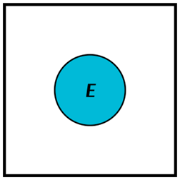
For example, let \(E\) be an event in which we roll a die and get 2 then this what the Venn diagram of the event looks like:

The Venn diagram for the complement of \(E\) can be easily derived from the Venn diagram of \(E\):

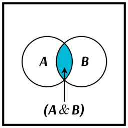
This is what the Venn diagram for the intersection of \(A\) and \(B\) looks like:
For example, let \(A\) be an event in which we roll a die and get anything but 1 with the following Venn diagram:

And let \(B\) be an event in which we roll a die and get a number less than 3 with the following Venn diagram:
The Venn diagram for the intersection of \(A\) and \(B\) can be easily derived from the Venn diagrams of \(A\) and \(B\):

This is what the Venn diagram for the union of \(A\) and \(B\) looks like:

For example, let \(A\) be an event in which we roll a die and get an even number with the following Venn diagram:

And let \(B\) be an event in which we roll a die and get a number less than 3 with the following Venn diagram:

The Venn diagram for the union of \(A\) and \(B\) can be easily derived from the Venn diagrams of A and B:

We learned how to visualize the events using the concept of a Venn diagram.
Section 3: Probability Rules
Next, we will discuss how to find the probabilities of compound events if the probability of the original event or events are given.
Mutually exclusive (or disjoint) events are the events that have no common outcomes.
- In the experiment of rolling a die with the well-known sample space, let \(A\) be an event \(\{1, 3\}\), \(B\) be an event \(\{4, 6\}\) and \(C\) be an event \(\{1, 3, 6\}\). \(A\) and \(B\) are said to be mutually exclusive or disjoint because they have no common outcomes. The same cannot be said about the events \(A\) and \(C\) or \(B\) and \(C\) because they share at least one common outcome.
- In the experiment of tossing two coins with the well-known sample space, let \(A\) be an event \(\{HH, HT\}\), \(B\) be an event \(\{HH, TT\}\) and \(C\) be an event \(\{TT\}\). \(A\) and \(C\) are said to be mutually exclusive or disjoint because they have no common outcomes. The same cannot be said about the events \(A\) and \(B\) or \(B\) and \(C\) because they share at least one common outcome.
A few more remarks about mutually exclusive events:
- A pair of events are mutually exclusive if their intersection is empty, and vice versa. This is the only way to find out whether a pair of events are mutually exclusive or not.
- An event \(E\) and its complement are mutually exclusive, because \(P(E and \bar{E})=0\).
The purpose of developing the probability rules is to be able to determine the probabilities of the complements, the union, and the intersection of events \(A\) and \(B\) from the probabilities of the event \(A\) and \(B\), that is we want to be able to find the probabilities of compound events if the probabilities of the original events are given.
Consider the union of two mutually exclusive events \(A\) and \(B\) as it is shown on the Venn diagram:
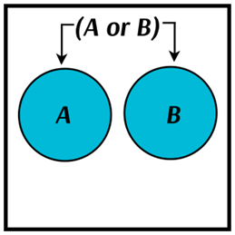
Recall that the areas of the regions represent the probabilities of the corresponding events. So the area of the union \(A\) and \(B\) is equal to the sum of the areas of \(A\) and area \(A\) in other words
\(P(A\text{ or }B)=P(A)+P(B)\)
This relation is called the special addition rule. What makes it special is the fact that it only applies to mutually exclusive events.
- If \(A\), \(B\) are disjoint and \(P(A)=0.2\), \(P(B)=0.5\) then \(P(A\text{ or }B)=0.2+0.5=0.7\).
- If \(C\), \(D\) are disjoint and \(P(C)=0.3\), \(P(D)=0.6\) then \(P(C\text{ or }D)=0.3+0.6=0.9\).
Consider the union of two events \(A\) and \(B\) that are not necessarily mutually exclusive as it is shown on the Venn diagram:

Notice that the special addition rule doesn’t work in this case because the combined area of \(A\) and \(B\) exceeds the area of the union. The good news is that we know exactly the difference between the two, so the area of the union \(A\) and \(B\) is equal to the sum of the areas of \(A\) and area \(B\) minus the area of the intersection, in other words:
\(P(A\text{ or }B)=P(A)+P(B)-P(A\text{ and }B)\)
This relation is called the general addition rule. What makes it general is the fact that it applies regardless of whether the events are mutually exclusive or not.
- If \(P(A\text{ and }B)=0.1\), \(P(A)=0.2\), \(P(B)=0.5\) then \(P(A\text{ or }B)=0.2+0.5-0.1=0.6\).
- If \(P(C\text{ and }D)=0.2\), \(P(C)=0.3\), \(P(D)=0.6\) then \(P(C\text{ or }D)=0.3+0.6-0.2=0.7\).
Finally, we will discuss the complementary rule.
Consider an event E and its complimentary event as it is shown on the Venn diagram:

Recall that the areas of the regions represent the probabilities of the corresponding events and since the total area is equal to 1 it is fair to say that
\(P(E)+P(\text{not }E)=1\)
This relation is called the complementary rule. We can use this relation to find the probability of the complementary event of \(E\) by subtracting the probability of \(E\) from 1.
- If \(P(\text{Rain})=0.2\) then \(P(\text{Not Rain})=1-0.2=0.8\).
- If \(P(\text{Late})=0.01\) then \(P(\text{Not Late})=1-0.01=0.99\).
We discussed the complementary rule, and the special and general addition rules that allow us to find the probability of the complementary event and the union of two events.