14.1: One-Way ANOVA

Next, we will learn how to apply the one-way analysis of variance to test a statistical claim about more than two population means.

A dean wants to check the consistency of teaching quality among the faculty in one of the departments. A sample of students was obtained from three classes taught by three different faculty, and their common final exam scores were recorded.

Class	Final Exam Scores
1	62	66	73	73	91	68	72
2	78	74	76	71	70	77	68	71
3	82	80	69	77	68	86

Use \(10\%\) significance level to test the claim that the teaching quality is consistent among the three courses.

Let’s compute the summaries for each sample:

Class	Final Exam Scores								\(\bar{x}_i\)	\(s_i\)	\(n_i\)
1	62	66	73	73	91	68	72		72.14	9.26	7
2	78	74	76	71	70	77	68	71	73.13	3.64	8
3	82	80	69	77	68	86			77.00	7.21	6

Let’s compute the summary of all sample combined:

Sample	\(\bar{x}_i\)	\(s_i\)	\(n_i\)
Combined	73.90	6.90	21

Now, let’s identify the statistical claim that needs to be tested:

“the teaching quality is consistent among the three courses”

A one way to measure the quality is by the average grade on the common exam thus we are testing the claim that

“all means are the same”

We can symbolically express the claim as

\(\mu_1=\mu_2=\mu_3\)

The way we are going to measure the likeliness of three samples is by computing the test statistic. But let’s gather some intuition about what we are trying to achieve. This is the distribution of all test results as if they were in one sample – we can call it the average distribution.

These are the graphs of three sample distributions that we obtained.

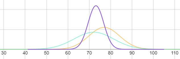
Do they look the same or in other words to they look like the average distribution? The answer is not obvious.

It would be an obvious “no” if they looked like this:

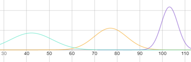
In such a case, we would expect the test statistic to be very high and if all distributions were overlapping the average distribution, then the answer will be an obvious “yes” and the test statistic will be equal to 0.

Let’s check if all necessary assumptions are satisfied:

• Simple random and independent samples
• Normal populations
• Equal population standard deviations

We will use the following template to perform the hypothesis testing:

In step 1, we will set up the hypothesis:

The null and alternative hypothesis are always the same in an ANOVA test. The null hypothesis is that the population means are the same and the alternative hypothesis is that at least one of the means is not the same as the others. The one-way ANOVA test is always (!) right-tail.

\(H_0\): all the means are equal \(H_a\): not all the means are equal

RT

In step 2, we will identify the significance level:

The significance level can always be found in the text of the problem. In our case it is \(10\%\), thus:

\(\alpha=0.10\)

In step 3, we will find the test statistic by finding the ratio of the variation between the samples and the variation within the samples:

\(f_0=\frac{\text{VAR}_{\text{between}}}{\text{VAR}_{\text{within}}}=\frac{42.04}{48.21}=0.872\)

The table summarizes all the computations necessary to compute the test statistic \(f_0\) which follows \(F\) distribution with \(dfn=k-1=2\) degrees of freedom in the numerator and \(dfd=n-k\) degrees of freedom in the denominator, where \(k=3\) is the number of samples and \(n=7+8+6=21\) is the size of all samples combined.

Sample Stats	Sample 1	Sample 2	Sample 3
Size (\(n_i\))	\(7\)	\(8\)	\(6\)	Mean (\(\bar{x}\))
Mean (\(\bar{x}_i\))	\(72.14\)	\(73.13\)	\(77.00\)	\(73.90\)
Variance (\(s^2_i\))	\(85.81\)	\(13.27\)	\(52.00\)
	\(n_i\)	\(\bar{x}_i\)	\(n_i\cdot(\bar{x}_i-\bar{x})^2\)
Sample 1	\(7\)	\(72.14\)	\(7\cdot(72.14-73.90)^2=\)	\(21.68\)
Sample 2	\(8\)	\(73.13\)	\(8\cdot(73.13-73.90)^2=\)	\(4.74\)
Sample 3	\(6\)	\(77.00\)	\(6\cdot(77.00-73.90)^2=\)	\(57.66\)
\(k-1=\)	\(3-1=2\)		\(\text{Total}_1=\)	\(84.08\)	\(\text{VAR}_{\text{between}}=\frac{\text{Total}_1}{k-1}=\frac{84.08}{2}=42.04\)
	\(n_i\)	\(s^2_i\)	\((n_i-1)\cdot s^2_i\)
Sample 1	\(7\)	\(85.81\)	\((7-1)\cdot85.81=\)	\(514.86\)
Sample 2	\(8\)	\(13.27\)	\((8-1)\cdot13.27=\)	\(92.89\)
Sample 3	\(6\)	\(52.00\)	\((6-1)\cdot52.00=\)	\(260\)
\(n-k=\)	\(21-3=18\)		\(\text{Total}_1=\)	\(867.75\)	\(\text{VAR}_{\text{within}}=\frac{\text{Total}_2}{n-k}=\frac{867.75}{18}=48.21\)

Try It Yourself!

In step 4, we will perform either the critical value approach or p-value approach to test the claim:

• In critical value approach, we construct the rejection region using the \(F\)-curve with \(dfn=k-1=3-1=2\) and \(dfd=n-k=21-3=18\), where \(n=21\) is the total number of observations in \(k=3\) samples:

RR: greater than \(f_{0.10}=2.624\)

Try It Yourself!

Try It Yourself!

• In p-value approach, we compute the p-value:

P-Value: \(P(F>0.872)=0.435\)

Try It Yourself!

In step 5, we will draw the conclusion:

• In the critical value approach, we must check whether the test statistic is in the rejection region or not. Our test statistic is \(0.872\) and it is to the left of the critical value \(2.624\), thus it is NOT in the rejection region.
• In the p-value approach, we must check whether the p-value is less than the significance level or not. Our p-value is \(0.435\) and it is greater than \(\alpha=0.10\).

Both tests suggest that we DO NOT reject the null hypothesis in favor of the alternative.

In step 6, we will interpret the results:

Under \(10\%\) significance level we DO NOT have sufficient evidence to suggest that the quality of teaching is inconsistent among the faculty in the department.

We discussed how to apply the ANOVA Procedure to test a statistical claim whether the population means are the same or not. This procedure is similar in spirit to the 2 means \(T\) POOLED procedure except that it can be done for three and more means.

Try It Yourself! \(\PageIndex{1}\)

Try It Yourself! \(\PageIndex{2}\)

Try It Yourself! \(\PageIndex{3}\)