5.4: Applications of Polynomials

Last updated
Save as PDF

Page ID: 51466

$ \newcommand{\vecs}[1]{\overset { \scriptstyle \rightharpoonup} {\mathbf{#1}} } $

$ \newcommand{\vecd}[1]{\overset{-\!-\!\rightharpoonup}{\vphantom{a}\smash {#1}}} $

$ \newcommand{\id}{\mathrm{id}}$ $ \newcommand{\Span}{\mathrm{span}}$

( \newcommand{\kernel}{\mathrm{null}\,}\) $ \newcommand{\range}{\mathrm{range}\,}$

$ \newcommand{\RealPart}{\mathrm{Re}}$ $ \newcommand{\ImaginaryPart}{\mathrm{Im}}$

$ \newcommand{\Argument}{\mathrm{Arg}}$ $ \newcommand{\norm}[1]{\| #1 \|}$

$ \newcommand{\inner}[2]{\langle #1, #2 \rangle}$

$ \newcommand{\Span}{\mathrm{span}}$

$ \newcommand{\id}{\mathrm{id}}$

$ \newcommand{\Span}{\mathrm{span}}$

$ \newcommand{\kernel}{\mathrm{null}\,}$

$ \newcommand{\range}{\mathrm{range}\,}$

$ \newcommand{\RealPart}{\mathrm{Re}}$

$ \newcommand{\ImaginaryPart}{\mathrm{Im}}$

$ \newcommand{\Argument}{\mathrm{Arg}}$

$ \newcommand{\norm}[1]{\| #1 \|}$

$ \newcommand{\inner}[2]{\langle #1, #2 \rangle}$

$ \newcommand{\Span}{\mathrm{span}}$ $ \newcommand{\AA}{\unicode[.8,0]{x212B}}$

$ \newcommand{\vectorA}[1]{\vec{#1}} % arrow$

$ \newcommand{\vectorAt}[1]{\vec{\text{#1}}} % arrow$

$ \newcommand{\vectorB}[1]{\overset { \scriptstyle \rightharpoonup} {\mathbf{#1}} } $

$ \newcommand{\vectorC}[1]{\textbf{#1}} $

$ \newcommand{\vectorD}[1]{\overrightarrow{#1}} $

$ \newcommand{\vectorDt}[1]{\overrightarrow{\text{#1}}} $

$ \newcommand{\vectE}[1]{\overset{-\!-\!\rightharpoonup}{\vphantom{a}\smash{\mathbf {#1}}}} $

$ \newcommand{\vecs}[1]{\overset { \scriptstyle \rightharpoonup} {\mathbf{#1}} } $

$ \newcommand{\vecd}[1]{\overset{-\!-\!\rightharpoonup}{\vphantom{a}\smash {#1}}} $

$\newcommand{\avec}{\mathbf a}$ $\newcommand{\bvec}{\mathbf b}$ $\newcommand{\cvec}{\mathbf c}$ $\newcommand{\dvec}{\mathbf d}$ $\newcommand{\dtil}{\widetilde{\mathbf d}}$ $\newcommand{\evec}{\mathbf e}$ $\newcommand{\fvec}{\mathbf f}$ $\newcommand{\nvec}{\mathbf n}$ $\newcommand{\pvec}{\mathbf p}$ $\newcommand{\qvec}{\mathbf q}$ $\newcommand{\svec}{\mathbf s}$ $\newcommand{\tvec}{\mathbf t}$ $\newcommand{\uvec}{\mathbf u}$ $\newcommand{\vvec}{\mathbf v}$ $\newcommand{\wvec}{\mathbf w}$ $\newcommand{\xvec}{\mathbf x}$ $\newcommand{\yvec}{\mathbf y}$ $\newcommand{\zvec}{\mathbf z}$ $\newcommand{\rvec}{\mathbf r}$ $\newcommand{\mvec}{\mathbf m}$ $\newcommand{\zerovec}{\mathbf 0}$ $\newcommand{\onevec}{\mathbf 1}$ $\newcommand{\real}{\mathbb R}$ $\newcommand{\twovec}[2]{\left[\begin{array}{r}#1 \\ #2 \end{array}\right]}$ $\newcommand{\ctwovec}[2]{\left[\begin{array}{c}#1 \\ #2 \end{array}\right]}$ $\newcommand{\threevec}[3]{\left[\begin{array}{r}#1 \\ #2 \\ #3 \end{array}\right]}$ $\newcommand{\cthreevec}[3]{\left[\begin{array}{c}#1 \\ #2 \\ #3 \end{array}\right]}$ $\newcommand{\fourvec}[4]{\left[\begin{array}{r}#1 \\ #2 \\ #3 \\ #4 \end{array}\right]}$ $\newcommand{\cfourvec}[4]{\left[\begin{array}{c}#1 \\ #2 \\ #3 \\ #4 \end{array}\right]}$ $\newcommand{\fivevec}[5]{\left[\begin{array}{r}#1 \\ #2 \\ #3 \\ #4 \\ #5 \\ \end{array}\right]}$ $\newcommand{\cfivevec}[5]{\left[\begin{array}{c}#1 \\ #2 \\ #3 \\ #4 \\ #5 \\ \end{array}\right]}$ $\newcommand{\mattwo}[4]{\left[\begin{array}{rr}#1 \amp #2 \\ #3 \amp #4 \\ \end{array}\right]}$ $\newcommand{\laspan}[1]{\text{Span}\{#1\}}$ $\newcommand{\bcal}{\cal B}$ $\newcommand{\ccal}{\cal C}$ $\newcommand{\scal}{\cal S}$ $\newcommand{\wcal}{\cal W}$ $\newcommand{\ecal}{\cal E}$ $\newcommand{\coords}[2]{\left\{#1\right\}_{#2}}$ $\newcommand{\gray}[1]{\color{gray}{#1}}$ $\newcommand{\lgray}[1]{\color{lightgray}{#1}}$ $\newcommand{\rank}{\operatorname{rank}}$ $\newcommand{\row}{\text{Row}}$ $\newcommand{\col}{\text{Col}}$ $\renewcommand{\row}{\text{Row}}$ $\newcommand{\nul}{\text{Nul}}$ $\newcommand{\var}{\text{Var}}$ $\newcommand{\corr}{\text{corr}}$ $\newcommand{\len}[1]{\left|#1\right|}$ $\newcommand{\bbar}{\overline{\bvec}}$ $\newcommand{\bhat}{\widehat{\bvec}}$ $\newcommand{\bperp}{\bvec^\perp}$ $\newcommand{\xhat}{\widehat{\xvec}}$ $\newcommand{\vhat}{\widehat{\vvec}}$ $\newcommand{\uhat}{\widehat{\uvec}}$ $\newcommand{\what}{\widehat{\wvec}}$ $\newcommand{\Sighat}{\widehat{\Sigma}}$ $\newcommand{\lt}{<}$ $\newcommand{\gt}{>}$ $\newcommand{\amp}{&}$ $\definecolor{fillinmathshade}{gray}{0.9}$

Learning Objectives

Geometric Applications
- Write a polynomial representing the perimeter of a shape
- Write a polynomial representing the area of a surface
- Write a polynomial representing the volume of a solid
Cost, Revenue, and Profit Polynomials
- Write a profit polynomial given revenue and cost polynomials
- Find profit for given quantities produced

In this section we will explore ways that polynomials are used in applications of perimeter, area, and volume. First, we will see how a polynomial can be used to describe the perimeter of a rectangle.

Example

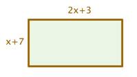
A rectangular garden has one side with a length of $2x + 3$. Find the perimeter of the garden.

$Rectangle with height x+7 and length 2x+3.$

[reveal-answer q=”627193″]Show Solution[/reveal-answer]
[hidden-answer a=”627193″]The perimeter of a rectangle is the sum of its side lengths.

$\left(x+7\right)+\left(2x+3\right)+\left(x+7\right)+\left(2x+3\right)$

Regroup by like terms.

$\left(x+2x+x+2x\right)+\left(7+3+7+3\right)$

Add like terms.

$6x+20$

Answer

The perimeter is $6x+20$.

[/hidden-answer]

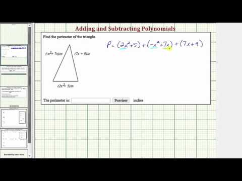
In the following video you are shown how to find the perimeter of a triangle whose sides are defined as polynomials.

$Thumbnail for the embedded element "Ex: Polynomial Addition Application - Perimeter"$

A YouTube element has been excluded from this version of the text. You can view it online here: pb.libretexts.org/ba/?p=106

The area of a circle can be found using the radius of the circle and the constant pi in the formula $A=\pi{r^2}$. In the next example we will use this formula to find a polynomial that describes the area of an irregular shape.

Example

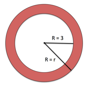
Find a polynomial for the shaded region of the figure.

$circle with middle extracted to form a ring shape. Inner radius labeled as r=3, outer radius labeled as R= r.$
[reveal-answer q=”667228″]Show Solution[/reveal-answer]
[hidden-answer a=”667228″]

Read and Understand: We need to find a way to describe the shaded region of this shape using polynomials. We know the formula for the area of a circle is $A=\pi{r^2}$. The figure we are working with is a circle with a smaller circle cut out.

Define and Translate: The larger circle has radius = r, and the smaller circle has radius= 3. If we find the area of the larger circle, then subtract the area of the smaller circle, the remaining area will be the shaded region. First define the area of the larger circle:

$A_{1}=\pi{r^2}$

Then define the area of the smaller circle.

$A_{2}=\pi{3^2}=9\pi$

Write and Solve: The shaded region can be found by subtracting the smaller area from the larger area.

$\begin{array}{c}A_{1}-A_{2}\\=\pi{r^2}-9\pi\end{array}$

The area of the shaded region is $\pi{r^2}-9\pi$

Answer

$\pi{r^2}-9\pi$

[/hidden-answer]

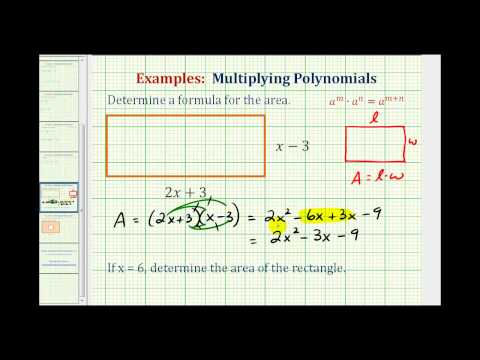
In the video that follows, you will be shown an example of determining the area of a rectangle whose sides are defined as polynomials.

$Thumbnail for the embedded element "Ex: Find the Area of a Rectangle Using a Polynomial"$

A YouTube element has been excluded from this version of the text. You can view it online here: pb.libretexts.org/ba/?p=106

$pi$

A note about pi.

It is easy to confuse pi as a variable because we use a greek letter to represent it. We use a greek letter instead of a number because nobody has been able to find an end to the number of digits of pi. To be precise and thorough, we use the greek letter as a way to say: “we are including all the digits of pi without having to write them”. The expression for the area of the shaded region in the example above included both the variable r, which represented an unknown radius and the number pi. If we needed to use this expression to build a physical object or instruct a machine to cut specific dimensions, we would round pi to an appropriate number of decimal places.

In the next example, we will write the area for a rectangle in two different ways, one as the product of two binomials and the other as the sum of four rectangles. Because we are describing the same shape two different ways, we should end up with the same expression no matter what way we define the area.

Example

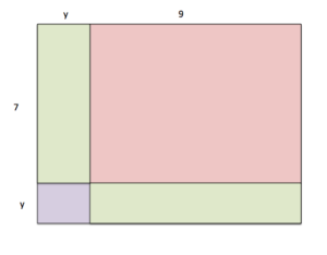
Write two different polynomials that describe the area of of the figure. For one expression, think of the rectangle as one large figure, and for the other expression, think of the rectangle as the sum of 4 different rectangles.

$Rectangle with side length y+9 and y+7$
[reveal-answer q=”15093″]Show Solution[/reveal-answer]
[hidden-answer a=”15093″]

First, we will define the polynomial that describes the area of the rectangle as one figure.

Read and Understand: We are tasked with writing an expressions for the area of the figure above. The area of a rectangle is given as $A=lw$. We need to consider the whole figure in our dimensions.

Define and Translate: Use the formula for area: $\begin{array}{c}l=\left(y+7\right)\\w=\left(y+9\right)\end{array}$

You could define $\begin{array}{c}w=\left(y+7\right)\\l=\left(y+9\right)\end{array}$ because it doesn’t matter in which order you multiply.

Write and Solve:

$\begin{array}{c}A=lw\\l=\left(y+7\right)\\w=\left(y+9\right)\end{array}$,

We can use either method we learned to multiply binomials to simplify this expression, we will use a table.

	$+7$
$y^2$	$+9$	$63$

Sum the terms from the table, and simplify:

$\begin{array}{c}\left(y+7\right)\left(y+9\right)\\=y^2+7y+9y+63\\=y^2+16y+63\end{array}$

Answer 1

$A=y^2+16y+63$

Now we will find an expression for the area of the whole figure as comprised by the areas of the four rectangles added together.

Read and Understand: The area of a rectangle is given as $A=lw$. We need to first define the areas of each rectangle, then sum them all together to get the area of the whole figure. It helps to label the four rectangle in the figure so you can keep the dimensions organized.

$Rectangle made from four rectangles labeled 1, 2, 3, 4.$

Define and Translate: Use the formula for area: $A=lw$ for each rectangle:

$A_{1}=7\cdot{y}$

$A_{2}=7\cdot{9}=63$

$A_{3}=y\cdot{y}=y^2$

$A_{4}=y\cdot{9}$

Write and Solve:

$\begin{array}{c}A=A_{1}+A_{2}+A_{3}+A_{4}\\=7y+63+y^2+9y\\\text{ reorganize and simplify }\\=y^2+16y+63\end{array}$

Answer 2

$A=y^2+16y+63$

Hopefully it isn;t surprising that both expressions simplify to the same thing.

[/hidden-answer]

The last example we will provide in this section is one for volume. The volume of regular solids such as spheres, cylinders, cones and rectangular prisms are known. We will find an expression for the volume of a cylinder, which is defined as $V=\pi{r^2}h$.

Example

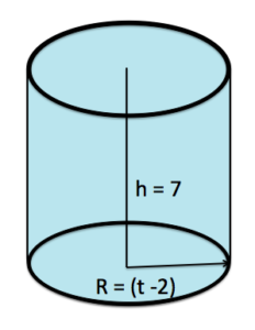
Define a polynomial that describes the volume of the cylinder shown in the figure:

$Cylinder with height = 7 and radius = (t-2)$
[reveal-answer q=”137608″]Show Solution[/reveal-answer]
[hidden-answer a=”137608″]

Read and Understand: We are tasked with writing an expressions for the volume of the cylinder in the figure above. The volume of a cylinder is given as$\pi$ is a constant, and r is the radius and h is the height of the cylinder.

Define and Translate: Use the formula for volume:$V=\pi{r^2}h$, we need to define r and h.

$\begin{array}{c}r=\left(t-2\right)\\h=7\end{array}$

Write and Solve: Substitute r and h into the formula for volume.

$\begin{array}{c}V=\pi{r^2}h\\=\pi\left(t-2\right)^2\cdot{7}\\=7\pi\left({t^2}-2t-2t+4\right)\\=7\pi\left({t^2}-4t+4\right)\end{array}$

Note that we usually write other constants that are multiplied by $7\pi$ to each term in the polynomial.

$\begin{array}{c}7\pi\left({t^2}-4t+4\right)\\=\left(7\pi\right){t^2}-\left(7\pi\right)\cdot{4t}+\left(7\pi\right)\cdot{4}\\=7\pi{t^2}-28\pi{t}+28\pi\end{array}$.

Note again how we left $\pi$ as a greek letter. If we needed to use this calculation for measurement of materials, we would round pi, or a computer would round for us.

Answer

$V=\pi{r^2}h=7\pi{t^2}-28\pi{t}+28\pi$

[/hidden-answer]

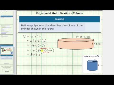
In this last video, we present another example of finding the volume of a cylinder whose dimensions include polynomials.

$Thumbnail for the embedded element "Polynomial Multiplication Application - Volume of a Cylinder"$

A YouTube element has been excluded from this version of the text. You can view it online here: pb.libretexts.org/ba/?p=106

Cost, Revenue, and Profit Polynomials

In the systems of linear equations section, we discussed how a company’s cost and revenue can be modeled with two linear equations. We found that the profit region for a company was the area between the two lines where the company would make money based on how much was produced. In this section, we will see that sometimes polynomials are used to describe cost and revenue.

Profit is typically defined in business as the difference between the amount of money earned (revenue) by producing a certain number of items and the amount of money it takes to produce that number of items. When you are in business, you definitely want to see profit, so it is important to know what your cost and revenue is.

$Pile of cell phones$

Cell Phones

For example, let’s say that the cost to a manufacturer to produce a certain number of things is C and the revenue generated by selling those things is R. The profit, P, can then be defined as

P = R-C

The example we will work with is a hypothetical cell phone manufacturer whose cost to manufacture x number of phones is $R=-0.09x^2+7000x$.

Example

Define a Profit polynomial for the hypothetical cell phone manufacturer.
[reveal-answer q=”50187″]Show Solution[/reveal-answer]
[hidden-answer a=”50187″]

Read and Understand: Profit is the difference between revenue and cost, so we will need to define P = R – C for the company.

Define and Translate: $\begin{array}{c}R=-0.09x^2+7000x\\C=2000x+750,000\end{array}$

Write and Solve: Substitute the expressions for R and C into the Profit equation.

$\begin{array}{c}P=R-C\\=-0.09x^2+7000x-\left(2000x+750,000\right)\\=-0.09x^2+7000x-2000x-750,000\\=-0.09x^2+5000x-750,000\end{array}$

Remember that when you subtract a polynomial, you have to subtract every term of the polynomial.

Answer

$P=-0.09x^2+5000x-750,000$

[/hidden-answer]

Mathematical models are great when you use them to learn important information. The cell phone manufacturing company can use the profit equation to find out how much profit they will make given x number of phones are manufactured. In the next example, we will explore some profit values for this company.

Example

Given the following numbers of cell phones manufactured, find the profit for the cell phone manufacturer:

x = 100 phones
x = 25,000 phones
x=60,000 phones

Interpret your results.
[reveal-answer q=”398706″]Show Solution[/reveal-answer]
[hidden-answer a=”398706″]

Read and Understand: The profit polynomial defined in the previous example,$P=-0.09x^2+5000x-750,000$, gives profit based on x number of phones manufactured. We need to substitute the given numbers of phones manufactured into the equation, then try to understand what our answer means in terms of profit and number of phones manufactured.

We will move straight into write and solve since we already have our polynomial. It is probably easiest to use a calculator since the numbers in this problem are so large.

Write and Solve:

Substitute x = 100

$\begin{array}{c}P=-0.09x^2+5000x-750,000\\=-0.09\left(100\right)^2+5000\left(100\right)-750,000\\=-900+500,000-750,000\\=-250,900\end{array}$

Interpret: When the number of phones manufactured is 100, the profit for the business is $-250,000. This is not what we want! The company must produce more than 100 phones to make a profit.

Write and Solve:

Substitute x = 25,000

$\begin{array}{c}P=-0.09x^2+5000x-750,000\\=-0.09\left(25000\right)^2+5000\left(25000\right)-750,000\\=-6120000+125,000,000-750,000\\=118,130,000\end{array}$

Interpret: When the number of phones manufactured is 25,000, the profit for the business is $118,130,000. This is more like it! If the company makes 25,000 phones it will make a profit after it pays all it’s bills.

If this is true, then the company should make even more phones so it can make even more money, right? Actually, something different happens as the number of items manufactured increases without bound.

Write and Solve:

Substitute x = 60,000

$\begin{array}{c}P=-0.09x^2+5000x-750,000\\=-0.09\left(60000\right)^2+5000\left(60000\right)-750,000\\=-324,000,000+300,000,000-750,000\\=-24,750,000\end{array}$

Interpret: When the number of phones manufactured is 60,000, the profit for the business is $-24,750,000. Wait a minute! If the company makes 60,000 phones it will lose money, what happened? At some point, the cost to manufacture the phones will overcome the amount of profit that the business can make. If this is interesting to you, you may enjoy reading about Economics and Business models.

[/hidden-answer]

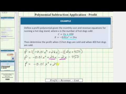
In the video that follows, we present another example of finding a polynomial profit equation.

$Thumbnail for the embedded element "Polynomial Subtraction App - Profit Equation from Revenue and Cost"$

A YouTube element has been excluded from this version of the text. You can view it online here: pb.libretexts.org/ba/?p=106

Summary

We have shown that profit can be modeled with a polynomial, and that the profit a company can make based on a business model like this has it’s bounds.

In this section we defined polynomials that represent perimeter, area and volume of well-known shapes. We also introduced some convention about how to use and write $\pi$ when it is combined with other constants and variables. The next application will introduce you to cost and revenue polynomials. We explored cost and revenue equations in the module on Systems of Linear Equations, now we will see that they can be more than just linear equations, they can be polynomials.

Screenshot PI. Provided by: Lumen Learning. License: CC BY: Attribution
Polynomial Multiplication Application - Volume of a Cylinder. Authored by: James Sousa (Mathispower4u.com) for Lumen Learning. Located at: https://youtu.be/g-g_nSsfGs4. License: CC BY: Attribution
Revision and Adaptation. Provided by: Lumen Learning. License: CC BY: Attribution
Polynomial Subtracton App - Profit Equation from Revene and Cost. Authored by: James Sousa (Mathispower4u.com) for Lumen Learning. Located at: https://youtu.be/-TWjDC4g9dU. License: CC BY: Attribution
Screenshot: Cell Phones. Provided by: Lumen Learning. License: CC BY: Attribution
Profit Polynomial Examples. Provided by: Lumen Learning. License: CC BY: Attribution

Ex: Polynomial Addition Application - Perimeter. Authored by: James Sousa (Mathispower4u.com). Located at: https://youtu.be/BhRpZv0_0jE. License: CC BY: Attribution
Ex: Find the Area of a Rectangle Using a Polynomial. Authored by: James Sousa (Mathispower4u.com) . Located at: https://youtu.be/5Q2htATOIik. License: CC BY: Attribution
Unit 11: Exponents and Polynomials, from Developmental Math: An Open Program. Provided by: Monterey Institute of Technology and Education. Located at: http://nrocnetwork.org/resources/downloads/nroc-math-open-textbook-units-1-12-pdf-and-word-formats/. License: CC BY: Attribution
Applied Optimization Problems. Provided by: OpenStax CNX. Located at: http://cnx.org/contents/svyieFe9@2/Applied-Optimization-Problems. License: CC BY-NC-SA: Attribution-NonCommercial-ShareAlike. License Terms: Download for free at http://cnx.org/contents/b2fca278-57b...21f539b4cc6f@2

	\(+7\)
\(y^2\)	\(+9\)	\(63\)

Search

Text Color

Text Size

Margin Size

Font Type

Answer

Answer 1

Answer 2

Answer

Answer