
13.2B: The Calculus of Vector-Valued Functions II


- Last updated
- Jun 5, 2019
- Save as PDF
( \newcommand{\kernel}{\mathrm{null}\,}\)
The previous section introduced us to a new mathematical object, the vector-valued function. We now apply calculus concepts to these functions. We start with the limit, then work our way through derivatives to integrals.
Limits of Vector-Valued Functions
The initial definition of the limit of a vector-valued function is a bit intimidating, as was the definition of the limit in Definition 1. The theorem following the definition shows that in practice, taking limits of vector-valued functions is no more difficult than taking limits of real-valued functions.
Definition 68: Limits of Vector-Valued Functions
Let I be an open interval containing c, and let ⇀r(t) be a vector-valued function defined on I, except possibly at c. The limit of ⇀r(t), as t approaches c, is ⇀L, expressed as
limt→c⇀r(t)=⇀L,
means that given any ϵ>0, there exists a δ>0 such that for all t≠c, if |t−c|<δ, we have ‖
Note how the measurement of distance between real numbers is the absolute value of their difference; the measure of distance between vectors is the vector norm, or magnitude, of their difference.
theorem 89: Limits of Vector-Valued Functions
- Let \vecs r(t) = \langle \,f(t),g(t)\,\rangle be a vector-valued function in \mathbb{R}^2 defined on an open interval I containing c. Then \lim_{t\to c} \vecs r(t) = \langle \lim_{t\to c}f(t)\, , \,\lim_{t\to c} g(t)\rangle.
- Let \vecs r(t) = \langle \,f(t),g(t),h(t)\,\rangle be a vector-valued function in \mathbb{R}^3 defined on an open interval I containing c. Then \lim_{t\to c} \vecs r(t) = \langle \lim_{t\to c}f(t)\, , \,\lim_{t\to c} g(t)\,, \,\lim_{t\to c} h(t)\rangle
Theorem 89 states that we compute limits component-wise.
Example \PageIndex{1}: Finding limits of vector-valued functions
Let \vecs r(t) = \langle \frac{\sin t}{t},\, t^2-3t+3,\,\cos t\rangle. Find \lim_{t\to 0}\vecs r(t).
Solution
We apply the theorem and compute limits component-wise.
\begin{align*} \lim_{t\to0} \vecs r(t) &= \langle \lim_{t\to 0}\frac{\sin t}{t}\, , \, \lim_{t\to 0} t^2-3t+3\, , \, \lim_{t\to 0} \cos t\rangle \\ &= \langle 1,3,1\rangle. \end{align*}
Continuity
Definition 69: Continuity of Vector-Valued Functions
Let \vecs r(t) be a vector-valued function defined on an open interval I containing c.
- \vecs r(t) is continuous at c if \lim_{t\to c} \vecs r(t) = r(c).
- If \vecs r(t) is continuous at all c in I, then \vecs r(t) is continuous on I.
We again have a theorem that lets us evaluate continuity component-wise.
THEOREM 90: Continuity of Vector-Valued Functions
Let \vecs r(t) be a vector-valued function defined on an open interval I containing c. \vecs r(t) is continuous at c if, and only if, each of its component functions is continuous at c.
Example \PageIndex{2}: Evaluating continuity of vector-valued functions
Let \vecs r(t) = \langle \frac{\sin t}{t},\, t^2-3t+3,\,\cos t\rangle. Determine whether \vecs r is continuous at t=0 and t=1.
Solution
While the second and third components of \vecs r(t) are defined at t=0, the first component, (\sin t)/t, is not. Since the first component is not even defined at t=0, \vecs r(t) is not defined at t=0, and hence it is not continuous at t=0.
At t=1 each of the component functions is continuous. Therefore \vecs r(t) is continuous at t=1.
Derivatives
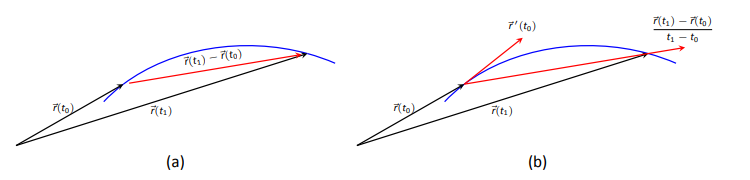
Consider a vector-valued function \vecs r defined on an open interval I containing t_0 and t_1. We can compute the displacement of \vecs r on [t_0,t_1], as shown in Figure \PageIndex{1a}. Recall that dividing the displacement vector by t_1-t_0 gives the average rate of change on [t_0,t_1], as shown in \PageIndex{1b}.
The derivative of a vector-valued function is a measure of the instantaneous rate of change, measured by taking the limit as the length of [t_0,t_1] goes to 0. Instead of thinking of an interval as [t_0,t_1], we think of it as [c,c+h] for some value of h (hence the interval has length h). The average rate of change is
\frac{\vecs r(c+h)-\vecs r(c)}{h}
for any value of h\neq0. We take the limit as h\to0 to measure the instantaneous rate of change; this is the derivative of \vecs r.
Definition 70: Derivative of a Vector-Valued Function
Let \vecs r(t) be continuous on an open interval I containing c.
- The derivative of \vecs r at t=c is \vecs r ^\prime (c) = \lim_{h\to 0} \frac{\vecs r(c+h) - \vecs r(c)}{h}.
- The derivative of \vecs r is \vecs r ^\prime (t) = \lim_{h\to 0} \frac{\vecs r(t+h) - \vecs r(t)}{h}.
Note: Alternate notations for the derivative of \vecs r include: \vecs r ^\prime(t) = \frac{d}{dt}\big(\,\vecs r(t)\,\big) = \frac{d\vecs r}{dt}.
If a vector-valued function has a derivative for all c in an open interval I, we say that \vecs r(t) is differentiable on I.
Once again we might view this definition as intimidating, but recall that we can evaluate limits component-wise. The following theorem verifies that this means we can compute derivatives component-wise as well, making the task not too difficult.
theorem 91: Derivatives of Vector-Valued Functions
- Let \vecs r(t) = \langle \, f(t), g(t)\,\rangle. Then \vecs r ^\prime(t) = \langle\, f^\prime (t), g^\prime (t)\, \rangle.
- Let \vecs r(t) = \langle \, f(t), g(t), h(t)\,\rangle. Then \vecs r ^\prime(t) = \langle\, f^\prime (t), g^\prime (t), h^\prime (t)\, \rangle.
Example \PageIndex{3}: Derivatives of vector-valued functions
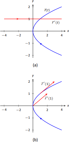
Let \vecs r(t) = \langle t^2,t\rangle.
- Sketch \vecs r(t) and \vecs r ^\prime(t) on the same axes.
- Compute \vecs r ^\prime(1) and sketch this vector with its initial point at the origin and at \vecs r(1).
Solution
- Theorem 91 allows us to compute derivatives component-wise, so \vecs r ^\prime(t) = \langle 2t, 1\rangle. \vecs r(t) and \vecs r ^\prime(t) are graphed together in Figure 11.9(a). Note how plotting the two of these together, in this way, is not very illuminating. When dealing with real-valued functions, plotting f(x) with f^\prime (x) gave us useful information as we were able to compare f and f^\prime at the same x-values. When dealing with vector-valued functions, it is hard to tell which points on the graph of \vecs r ^\prime correspond to which points on the graph of \vecs r.
- We easily compute \vecs r ^\prime(1) = \langle 2,1\rangle, which is drawn in Figure \PageIndex{2a} with its initial point at the origin, as well as at \vecs r(1) = \langle 1,1\rangle. These are sketched in Figure \PageIndex{2b}.
Example \PageIndex{4}: Derivatives of vector-valued functions
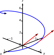
Let \vecs r(t) = \langle \cos t, \sin t, t\rangle. Compute \vecs r ^\prime(t) and \vecs r ^\prime(\pi/2). Sketch \vecs r ^\prime(\pi/2) with its initial point at the origin and at \vecs r(\pi/2).
Solution
We compute \vecs r ^\prime as \vecs r ^\prime(t) = \langle -\sin t, \cos t, 1\rangle. At t= \pi/2, we have \vecs r ^\prime(\pi/2) = \langle -1,0,1\rangle. Figure \PageIndex{3} shows a graph of \vecs r(t), with \vecs r ^\prime(\pi/2) plotted with its initial point at the origin and at \vecs r(\pi/2).
In Examples \PageIndex{3} and \PageIndex{4}, sketching a particular derivative with its initial point at the origin did not seem to reveal anything significant. However, when we sketched the vector with its initial point on the corresponding point on the graph, we did see something significant: the vector appeared to be tangent to the graph. We have not yet defined what "tangent'' means in terms of curves in space; in fact, we use the derivative to define this term.
Definition 71: Tangent Vector, Tangent Line
Let \vecs r(t) be a differentiable vector-valued function on an open interval I containing c, where \vecs r ^\prime(c)\neq \vecs 0.
- A vector \vecs v is tangent to the graph of \vecs r(t) at t=c if \vecs v is parallel to \vecs r ^\prime(c).
- The tangent line to the graph of \vecs r(t) at t=c is the line through \vecs r(c) with direction parallel to \vecs r ^\prime(c). An equation of the tangent line is
\vecs \ell(t) = \vecs r(c) + t\,\vecs r ^\prime(c).
Example \PageIndex{5}: Finding tangent lines to curves in space
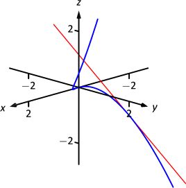
Let \vecs r(t) = \langle t,t^2,t^3\rangle on [-1.5,1.5]. Find the vector equation of the line tangent to the graph of \vecs r at t=-1.
Solution
To find the equation of a line, we need a point on the line and the line's direction. The point is given by \vecs r(-1) = \langle -1,1,-1\rangle. (To be clear, \langle -1,1,-1\rangle is a vector, not a point, but we use the point "pointed to'' by this vector.)
The direction comes from \vecs r ^\prime(-1). We compute, component-wise, \vecs r ^\prime(t) = \langle 1,2t, 3t^2\rangle. Thus \vecs r ^\prime(-1) = \langle 1,-2,3\rangle.
The vector equation of the line is \ell(t) = \langle -1,1,-1\rangle + t\langle 1,-2,3\rangle. This line and \vecs r(t) are sketched, from two perspectives, in Figure \PageIndex{4a} and \PageIndex{4b}.
Example \PageIndex{6}: Finding tangent lines to curves
Find the equations of the lines tangent to \vecs r(t) = \langle t^3,t^2\rangle at t=-1 and t=0.
Solution
We find that \vecs r ^\prime(t) = \langle 3t^2,2t\rangle. At t=-1, we have
\vecs r(-1) = \langle -1,1\rangle\quad \text{and}\quad \vecs r ^\prime(-1) = \langle 3,-2\rangle, \nonumber
so the equation of the line tangent to the graph of \vecs r(t) at t=-1 is
\ell(t) = \langle -1,1\rangle + t\langle 3,-2\rangle. \nonumber
This line is graphed with \vecs r(t) in Figure \PageIndex{5}.
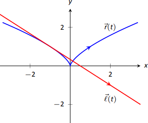
At t=0, we have \vecs r ^\prime(0) = \langle 0,0\rangle=\vecs 0! This implies that the tangent line "has no direction.'' We cannot apply Definition 71, hence cannot find the equation of the tangent line.
We were unable to compute the equation of the tangent line to \vecs r(t)= \langle t^3,t^2\rangle at t=0 because \vecs r ^\prime(0) = \vecs 0. The graph in Figure 11.12 shows that there is a cusp at this point. This leads us to another definition of smooth, previously defined by Definition 46 in Section 9.2.
Definition 72: Smooth Vector-Valued Functions
Let \vecs r(t) be a differentiable vector-valued function on an open interval I. \vecs r(t) is smooth on I if \vecs r ^\prime(t)\neq \vecs 0 on I.
Having established derivatives of vector-valued functions, we now explore the relationships between the derivative and other vector operations. The following theorem states how the derivative interacts with vector addition and the various vector products.
THEOREM 92: Properties of Derivatives of Vector-Valued Functions
Let \vecs r and \vecs s be differentiable vector-valued functions, let f be a differentiable real-valued function, and let c be a real number.
- \frac{d}{dt}\Big(\vecs r(t) \pm \vecs s(t)\Big) = \vecs r ^\prime(t) \pm \vecs s\,'(t)
- \frac{d}{dt}\Big(c\vecs r(t)\Big) = c\vecs r ^\prime(t)
- \frac{d}{dt}\Big(f(t)\vecs r(t)\Big) = f^\prime (t)\vecs r(t) + f(t)\vecs r ^\prime(t) Product Rule
- \frac{d}{dt}\Big(\vecs r(t)\cdot \vecs s(t) \Big) = \vecs r ^\prime(t)\cdot \vecs s(t) + \vecs r(t)\cdot \vecs s\,'(t) Product Rule
- \frac{d}{dt}\Big(\vecs r(t)\times \vecs s(t) \Big) = \vecs r ^\prime(t)\times \vecs s(t) + \vecs r(t)\times \vecs s\,'(t) Product Rule
- \frac{d}{dt}\Big(\vecs r\big(f(t)\big)\Big) = \vecs r ^\prime\big(f(t)\big)f^\prime (t) Chain Rule
Example \PageIndex{7}: Using derivative properties of vector-valued functions
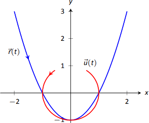
Let \vecs r(t) = \langle t, t^2-1\rangle and let \vecs u(t) be the unit vector that points in the direction of \vecs r(t).
- Graph \vecs r(t) and \vecs u(t) on the same axes, on [-2,2].
- Find \vecs u\,'(t) and sketch \vecs u\,'(-2), \vecs u\,'(-1) and \vecs u\,'(0). Sketch each with initial point the corresponding point on the graph of \vecs u.
Solution
- To form the unit vector that points in the direction of \vecs r, we need to divide \vecs r(t) by its magnitude.
\norm{\vecs r(t)} = \sqrt{t^2+(t^2-1)^2} \quad \Rightarrow \quad \vecs u(t) = \frac{1}{\sqrt{t^2+(t^2-1)^2}}\langle t,t^2-1\rangle.
\vecs r(t) and \vecs u(t) are graphed in Figure 11.13. Note how the graph of \vecs u(t) forms part of a circle; this must be the case, as the length of \vecs u(t) is 1 for all t. - To compute \vecs u\,'(t), we use Theorem 92, writing \vecs u(t) = f(t)\vecs r(t),\quad \text{where}\quad f(t) = \frac{1}{\sqrt{t^2+(t^2-1)^2}}=\big(t^2+(t^2-1)^2\big)^{-1/2}.
(We could write \vecs u(t) = \langle \frac{t}{\sqrt{t^2+(t^2-1)^2}}, \frac{t^2-1}{\sqrt{t^2+(t^2-1)^2}}\rangle
and then take the derivative. It is a matter of preference; this latter method requires two applications of the Quotient Rule where our method uses the Product and Chain Rules.)
We find f^\prime (t) using the Chain Rule: \begin{align*}f^\prime (t) &= -\frac12\big(t^2+(t^2-1)^2\big)^{-3/2}\big(2t+2(t^2-1)(2t)\big)\\&= -\frac{2t(2t^2-1)}{2\big(\sqrt{t^2+(t^2-1)^2}\,\big)^3}\end{align*}
We now find \vecs u\,'(t) using part 3 of Theorem 92: \begin{align*}\vecs u\,'(t) &= f^\prime (t)\vecs u(t) + f(t)\vecs u\,'(t) \\&= -\frac{2t(2t^2-1)}{2\big(\sqrt{t^2+(t^2-1)^2}\,\big)^3}\langle t,t^2-1\rangle + \frac{1}{\sqrt{t^2+(t^2-1)^2}}\langle 1,2t\rangle.\end{align*}
This is admittedly very "messy;'' such is usually the case when we deal with unit vectors. We can use this formula to compute \vecs u\,(-2), \vecs u\,(-1) and \vecs u\,(0): \begin{align*}\vecs u\,(-2) &= \langle -\frac{15}{13 \sqrt{13}},-\frac{10}{13\sqrt{13}}\rangle \approx \langle -0.320,-0.213\rangle\\\vecs u\,(-1) &= \langle 0,-2\rangle\\\vecs u\,(0) &= \langle 1,0\rangle\end{align*}
Each of these is sketched in Figure \PageIndex{6}. Note how the length of the vector gives an indication of how quickly the circle is being traced at that point. When t=-2, the circle is being drawn relatively slow; when t=-1, the circle is being traced much more quickly.
It is a basic geometric fact that a line tangent to a circle at a point P is perpendicular to the line passing through the center of the circle and P. This is illustrated in Figure 11.14; each tangent vector is perpendicular to the line that passes through its initial point and the center of the circle. Since the center of the circle is the origin, we can state this another way: \vecs u\,'(t) is orthogonal to \vecs u(t).
Recall that the dot product serves as a test for orthogonality: if \vecs u\cdot \vecs v = 0, then \vecs u is orthogonal to \vecs v. Thus in the above example, \vecs u(t)\cdot \vecs u\,'(t)=0.
This is true of any vector-valued function that has a constant length, that is, that traces out part of a circle. It has important implications later on, so we state it as a theorem (and leave its formal proof as an Exercise.)
THEOREM 93 Vector-Valued Functions of Constant Length
Let \vecs r(t) be a differentiable vector-valued function on an open interval I of constant length. That is, \norm{\vecs r(t)} = c for all t in I (equivalently, \vecs r(t)\cdot \vecs r(t) = c^2 for all t in I). Then \vecs r(t)\cdot\vecs r ^\prime(t) = 0 for all t in I.
Integration
Indefinite and definite integrals of vector-valued functions are also evaluated component-wise.
THEOREM 94: Indefinite and Definite Integrals of Vector-Valued Functions
Let \vecs r(t) = \langle f(t),g(t)\rangle be a vector-valued function in \mathbb{R}^2.
- \int \vecs r(t)\ dt = \langle \int f(t)\ dt, \int g(t)\ dt\rangle
- \int_a^b \vecs r(t)\ dt = \langle \int_a^b f(t)\ dt, \int_a^b g(t)\ dt\rangle
A similar statement holds for vector-valued functions in \mathbb{R}^3.
Example \PageIndex{8}: Evaluating a definite integral of a vector-valued function
Let \vecs r(t) = \langle e^{2t},\sin t\rangle. Evaluate \int_0^1 \vecs r(t) \ dt.
Solution
We follow Theorem 94.
\begin{align*} \int_0^1 \vecs r(t) \ dt &= \int_0^1 \langle e^{2t},\sin t\rangle \ dt \\ &= \langle \int_0^1 e^{2t}\ dt\ , \int_0^1 \sin t \ dt \rangle \\ &= \langle \frac12e^{2t}\Big|_0^1\ , -\cos t\Big|_0^1\rangle \\ &= \langle \frac12(e^2-1)\ , -\cos(1)+1\rangle\\ &\approx \langle 3.19,0.460\rangle. \end{align*}
Example \PageIndex{9}: Solving an initial value problem
Let \vecs r ^{\prime\prime}(t) = \langle 2, \cos t, 12t\rangle. Find \vecs r(t) where:
- \vecs r(0) = \langle -7,-1,2\rangle and
- \vecs r ^\prime(0) = \langle 5,3,0\rangle.
Solution
Knowing \vecs r ^{\prime\prime}(t) = \langle 2,\cos t, 12t\rangle, we find \vecs r ^\prime(t) by evaluating the indefinite integral.
\begin{align*} \int \vecs r ^{\prime\prime}(t) dt &= \langle \int 2 dt\ , \int \cos t dt\ , \int 12t dt\rangle \\ &= \langle 2t+C_1, \sin t+ C_2, 6t^2 + C_3\rangle \\ &= \langle 2t,\sin t,6t^2 \rangle + \langle C_1,C_2,C_3\rangle \\ &= \langle 2t,\sin t,6t^2 \rangle + \vecs C_1. \end{align*}
Note how each indefinite integral creates its own constant which we collect as one constant vector \vecs C_1. Knowing \vecs r ^\prime(0) = \langle 5,3,0\rangle allows us to solve for \vecs C_1:
\begin{align*} \vecs r ^\prime(t) & = \langle 2t,\sin t,6t^2 \rangle + \vecs C_1\\ \vecs r ^\prime(0) &= \langle 0,0,0 \rangle + \vecs C_1\\ \langle 5,3,0\rangle &= \vecs C_1. \end{align*}
So \vecs r ^\prime(t) = \langle 2t,\sin t,6t^2\rangle + \langle 5,3,0\rangle = \langle 2t+5, \sin t + 3, 6t^2\rangle. To find \vecs r(t), we integrate once more.
\begin{align*} \int \vecs r ^\prime(t)\ dt &= \langle \int 2t+5\ dt, \int \sin t + 3\ dt, \int 6t^2 dt \rangle\\ &= \langle t^2+5t, -\cos t + 3t, 2t^3\rangle + \vecs C_2. \end{align*}
With \vecs r(0) = \langle -7,-1,2\rangle, we solve for \vecs C_2:
\begin{align*}
\vecs r(t) &= \langle t^2+5t, -\cos t + 3t, 2t^3\rangle + \vecs C_2\\
\vecs r(0) &= \langle 0,-1,0\rangle + \vecs C_2\\
\langle -7,-1,2\rangle &= \langle 0,-1,0\rangle + \vecs C_2\\
\langle -7,0,2\rangle &= \vecs C_2.
\end{align*}
So \vecs r(t) = \langle t^2+5t, -\cos t + 3t, 2t^3\rangle + \langle -7,0,2\rangle = \langle t^2+5t-7,-\cos t+3t,2t^3+2\rangle.
What does the integration of a vector-valued function mean? There are many applications, but none as direct as "the area under the curve'' that we used in understanding the integral of a real-valued function.
A key understanding for us comes from considering the integral of a derivative: \int_a^b \vecs r ^\prime(t) dt = \vecs r(t)\Big|_a^b = \vecs r(b)-\vecs r(a).
Integrating a rate of change function gives displacement.
Noting that vector-valued functions are closely related to parametric equations, we can describe the arc length of the graph of a vector-valued function as an integral. Given parametric equations x=f(t), y=g(t), the arc length on [a,b] of the graph is
\text{Arc Length} = \int_a^b\sqrt{f^\prime (t)^2+g^\prime (t)^2} dt,
as stated in Theorem 82 in Section 9.3. If \vecs r (t) = \langle f(t), g(t)\rangle, note that \sqrt{f^\prime (t)^2+g^\prime (t)^2} = \norm{\vecs r ^\prime(t)}. Therefore we can express the arc length of the graph of a vector-valued function as an integral of the magnitude of its derivative.
THEOREM 95: Arc Length of a Vector-Valued Function
Let \vecs r (t) be a vector-valued function where \vecs r ^\prime(t) is continuous on [a,b]. The arc length L of the graph of \vecs r (t) is L = \int_a^b \norm{\vecs r ^\prime(t)}\ dt.
Note that we are actually integrating a scalar-function here, not a vector-valued function.
The next section takes what we have established thus far and applies it to objects in motion. We will let \vecs r (t) describe the path of an object in the plane or in space and will discover the information provided by \vecs r ^\prime(t) and \vecs r ^{\prime\prime}(t).