7.5: Constant Coefficient Equations with Piecewise Continuous Forcing Functions

We’ll now consider initial value problems of the form

\[\label{eq:8.5.1} ay''+by'+cy=f(t), \quad y(0)=k_0,\quad y'(0)=k_1,\]

where \(a\), \(b\), and \(c\) are constants (\(a\ne0\)) and \(f\) is piecewise continuous on \([0,\infty)\). Problems of this kind occur in situations where the input to a physical system undergoes instantaneous changes, as when a switch is turned on or off or the forces acting on the system change abruptly.

It can be shown (Exercises 8.5.23 and 8.5.24) that the differential equation in Equation \ref{eq:8.5.1} has no solutions on an open interval that contains a jump discontinuity of \(f\). Therefore we must define what we mean by a solution of Equation \ref{eq:8.5.1} on \([0,\infty)\) in the case where \(f\) has jump discontinuities. The next theorem motivates our definition. We omit the proof.

Theorem \(\PageIndex{1}\)

Suppose \(a,b\), and \(c\) are constants \((a\ne0),\) and \(f\) is piecewise continuous on \([0,\infty).\) with jump discontinuities at \(t_1,\) …, \(t_n,\) where

\[0<t_1<\cdots<t_n. \nonumber\]

Let \(k_0\) and \(k_1\) be arbitrary real numbers. Then there is a unique function \(y\) defined on \([0,\infty)\) with these properties:

1. \(y(0)=k_0\) and \(y'(0)=k_1\).
2. \(y\) and \(y'\) are continuous on \([0,\infty)\).
3. \(y''\) is defined on every open subinterval of \([0,\infty)\) that does not contain any of the points \(t_1,\) …, \(t_n\), and \[ay''+by'+cy=f(t) \nonumber\] on every such subinterval.
4. \(y''\) has limits from the right and left at \(t_1,\) …\(,\) \(t_n\).

We define the function \(y\) of Theorem \(\PageIndex{1}\) to be the solution of the initial value problem Equation \ref{eq:8.5.1}.

We begin by considering initial value problems of the form

\[\label{eq:8.5.2} ay''+by'+cy=\left\{\begin{array}{cl} f_0(t),&0\le t<t_1,\\[4pt]f_1(t),&t\ge t_1, \end{array}\right.\quad y(0)=k_0,\quad y'(0)=k_1,\]

where the forcing function has a single jump discontinuity at \(t_1\).

Howto: Solve Constant Coefficient Equations with Piecewise Continuous Forcing Functions

We can solve Equation \ref{eq:8.5.2} by the these steps:

• Step 1. Find the solution \(y_0\) of the initial value problem \[ay''+by'+cy=f_0(t), \quad y(0)=k_0,\quad y'(0)=k_1. \nonumber \]
• Step 2. Compute \(c_0=y_0(t_1)\) and \(c_1=y_0'(t_1)\).
• Step 3. Find the solution \(y_1\) of the initial value problem \[ay''+by'+cy=f_1(t), \quad y(t_1)=c_0,\quad y'(t_1)=c_1.\nonumber\]
• Step 4. Obtain the solution \(y\) of Equation \ref{eq:8.5.2} as \[y=\left\{\begin{array}{cl} y_0(t),&0\le t<t_1\\[4pt]y_1(t),&t\ge t_1. \end{array}\right.\nonumber\]

It is shown in Exercise 8.5.23 that \(y'\) exists and is continuous at \(t_1\). The next example illustrates this procedure.

Example \(\PageIndex{1}\)

Solve the initial value problem

\[\label{eq:7.5.3} y''+y=f(t), \quad y(0)=2,\; y'(0)=-1,\]

where

\[f(t)=\left\{\begin{array}{rl} 1,&0\le t< {\pi\over2},\\[4pt] -1,&t\ge {\pi\over2}. \end{array}\right. \nonumber\]

Figure \(\PageIndex{1}\): Graph of Equation \ref{eq:8.5.4}

Solution

The initial value problem in Step 1 is

\[y''+y=1, \quad y(0)=2,\quad y'(0)=-1. \nonumber\]

We leave it to you to verify that its solution is

\[y_0=1+\cos t-\sin t. \nonumber\]

Doing Step 2 yields \(y_0(\pi/2)=0\) and \(y_0'(\pi/2)=-1\), so the second initial value problem is

\[y''+y=-1, \quad y\left({\pi\over2}\right)=0,\; y'\left({\pi\over 2}\right)=-1. \nonumber\]

We leave it to you to verify that the solution of this problem is

\[y_1=-1+\cos t+\sin t. \nonumber\]

Hence, the solution of Equation \ref{eq:8.5.3} is

\[\label{eq:8.5.4} y=\left\{\begin{array}{rl} 1+\cos t-\sin t,&0\le t< {\pi\over2}, \\[4pt] -1+\cos t+\sin t,&t\ge {\pi\over2} \end{array}\right.\]

If \(f_0\) and \(f_1\) are defined on \([0,\infty)\), we can rewrite Equation \ref{eq:8.5.2} as

\[ay''+by'+cy=f_0(t)+u(t-t_1)\left(f_1(t)-f_0(t)\right), \quad y(0)=k_0,\quad y'(0)=k_1, \nonumber\]

and apply the method of Laplace transforms. We’ll now solve the problem considered in Example [example:8.5.1} by this method.

Example \(\PageIndex{2}\)

Use the Laplace transform to solve the initial value problem

\[\label{eq:8.5.5} y''+y=f(t), \quad y(0)=2,\; y'(0)=-1,\]

where

\[f(t)=\left \{ \begin{array}{cl} \phantom{-}1,&0\le t< {\pi\over2},\\ -1,&t \ge {\pi\over2}. \end{array}\right. \nonumber\]

Solution

Here

\[f(t)=1-2u\left(t-{\pi\over2}\right), \nonumber\]

so Theorem \(\PageIndex{1}\) (with \(g(t)=1\)) implies that

\[{\cal L}(f)={1-2e^{-{\pi s/2}}\over s}. \nonumber\]

Therefore, transforming Equation \ref{eq:8.5.5} yields

\[(s^2+1)Y(s)={1-2e^{-{\pi s/ 2}}\over s}-1+2s, \nonumber\]

so

\[\label{eq:8.5.6} Y(s)=(1-2e^{-{\pi s/ 2}}) G(s)+{2s-1\over s^2+1},\]

with

\[G(s)={1\over s(s^2+1)}. \nonumber\]

The form for the partial fraction expansion of \(G\) is

\[\label{eq:8.5.7} {1\over s(s^2+1)}={A\over s}+{Bs+C\over s^2+1}. \]

Multiplying through by \(s(s^2+1)\) yields

\[A(s^2+1)+(Bs+C)s=1, \nonumber\]

or

\[(A+B)s^2+Cs+A=1. \nonumber\]

Equating coefficients of like powers of \(s\) on the two sides of this equation shows that \(A=1\), \(B=-A=-1\) and \(C=0\). Hence, from Equation \ref{eq:8.5.7},

\[G(s)={1\over s}-{s\over s^2+1}. \nonumber\]

Therefore

\[g(t)=1-\cos t. \nonumber\]

From this, Equation \ref{eq:8.5.6}, and Theorem 8.4.2,

\[y=1-\cos t-2u\left(t-{\pi\over2}\right)\left(1-\cos\left(t-{\pi \over2}\right)\right)+2\cos t-\sin t. \nonumber\]

Simplifying this (recalling that \(\cos (t-\pi/2)=\sin t)\) yields

\[y=1+\cos t-\sin t-2u\left(t-{\pi\over2}\right)(1-\sin t), \nonumber\]

or

\[y=\left\{\begin{array}{cl}{1+\cos t-\sin t,}&{0\leq t<\frac{\pi }{2}}\\{-1+\cos t+\sin t,}&{t\geq \frac{\pi }{2}} \end{array} \right.\nonumber \]

which is the result obtained in Example \(\PageIndex{1}\).

Note

It isn’t obvious that using the Laplace transform to solve Equation \ref{eq:8.5.2} as we did in Example \(\PageIndex{2}\) yields a function \(y\) with the properties stated in Theorem \(\PageIndex{1}\); that is, such that \(y\) and \(y'\) are continuous on \([0, ∞)\) and \(y''\) has limits from the right and left at \(t_{1}\). However, this is true if \(f_{0}\) and \(f_{1}\) are continuous and of exponential order on \([0, ∞)\). A proof is sketched in Exercises 8.6.11–8.6.13.

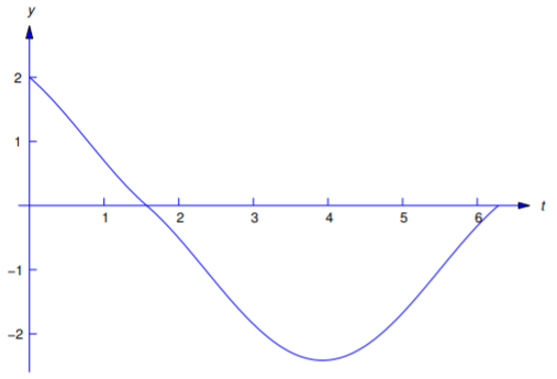
Example \(\PageIndex{3}\)

Solve the initial value problem

\[\label{eq:8.5.8} y''-y=f(t), \quad y(0)=-1,\; y'(0)=2,\]

where

\[f(t)=\left\{\begin{array}{cl} t,&0\le t<1,\\ 1,&t\ge 1. \end{array}\right.\nonumber\]

Solution

Here

\[f(t)=t-u(t-1)(t-1),\nonumber\]

so

\[\begin{align*} {\cal L}(f)&={\cal L}(t)-{\cal L}\left(u(t-1)(t-1)\right)\\[4pt] &=\cal L(t)-e^{-s}{\cal L}(t)\text{ (from Theorem 8.4.1})\\[4pt] &={1\over s^2}-{e^{-s}\over s^2}.\end{align*}\nonumber\]

Since transforming Equation \ref{eq:8.5.8} yields

\[(s^2-1) Y(s)={\cal L}(f)+2-s,\nonumber\]

we see that

\[\label{eq:8.5.9} Y(s)=(1-e^{-s})H(s)+{2-s\over s^2-1},\]

where

\[H(s)={1\over s^2(s^2-1)}={1\over s^2-1}-{1\over s^2};\nonumber\]

therefore

\[\label{eq:8.5.10} h(t)=\sinh t-t.\]

Since

\[{\cal L}^{-1}\left({2-s\over s^2-1}\right)=2\sinh t-\cosh t,\nonumber\]

we conclude from Equation \ref{eq:8.5.9}, Equation \ref{eq:8.5.10}, and Theorem \(\PageIndex{1}\) that

\[y=\sinh t-t-u(t-1)\left(\sinh (t-1)-t+1\right)+2\sinh t- \cosh t,\nonumber\]

or

\[\label{eq:8.5.11} y=3\sinh t-\cosh t-t-u(t-1)\left(\sinh (t-1)-t+1\right)\]

We leave it to you to verify that \(y\) and \(y'\) are continuous and \(y''\) has limits from the right and left at \(t_1=1\).

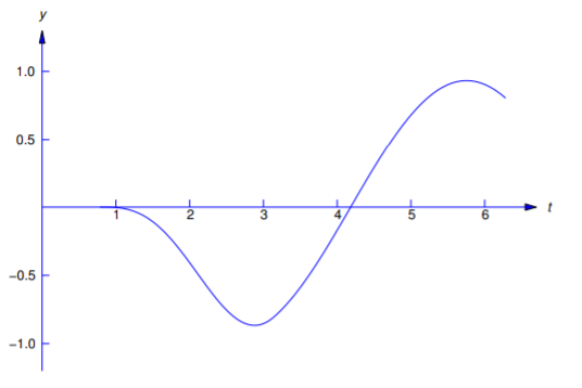
Example \(\PageIndex{4}\)

Solve the initial value problem

\[\label{eq:8.5.12} y''+y=f(t), \quad y(0)=0,\; y'(0)=0,\]

where

\[f(t)=\left\{\begin{array}{cl}{0,}&{0\leq t<\frac{\pi }{4}}\\{\cos 2t}&{\frac{\pi }{4}\leq t< \pi }\\{0,}&{t\geq \pi } \end{array} \right.\nonumber \]

Solution

Here

\[f(t)=u(t-\pi/4)\cos2t-u(t-\pi)\cos2t, \nonumber\]

so

\[\begin{align*} {\cal L}(f)&={\cal L}\left(u(t-\pi/4)\cos2t\right)-{\cal L}\left( u(t-\pi)\cos2t\right)\\[4pt] &=e^{-{\pi s/4}}{\cal L}\left(\cos2(t+\pi/4)\right)-e^{-\pi s} {\cal L}\left(\cos2(t+\pi)\right)\\[4pt] &=-e^{-{\pi s/4}}{\cal L}(\sin2t)-e^{-\pi s} {\cal L}(\cos2t)\\[4pt] &=-{2e^{-{\pi s/ 4}}\over s^2+4}-{se^{-\pi s}\over s^2+4}.\end{align*}\nonumber\]

Since transforming Equation \ref{eq:8.5.12} yields

\[(s^2+1)Y(s)={\cal L}(f),\nonumber\]

we see that

\[\label{eq:8.5.13} Y(s)=e^{-{\pi s/ 4}} H_1(s)+e^{-\pi s} H_2(s),\]

where

\[\label{eq:8.5.14} H_1(s)=-{2\over (s^2+1)(s^2+4)}\quad\mbox{ and }\quad H_2(s)=-{s \over (s^2+1)(s^2+4)}.\]

To simplify the required partial fraction expansions, we first write

\[{1\over (x+1)(x+4)}={1\over3}\left[{1\over x+1}-{1\over x+4}\right].\nonumber\]

Setting \(x=s^2\) and substituting the result in Equation \ref{eq:8.5.14} yields

\[H_1(s)=-{2\over3}\left[{1\over s^2+1}-{1\over s^2+4}\right] \quad\mbox{ and }\quad H_2(s)=-{1\over3}\left[{s\over s^2+1}-{s\over s^2+4}\right].\nonumber\]

The inverse transforms are

\[h_1(t)=-{2\over3}\sin t+{1\over3}\sin2t \quad\mbox{ and }\; h_2(t)=-{1\over3}\cos t+{1\over3}\cos2t.\nonumber\]

From Equation \ref{eq:8.5.13} and Theorem 8.4.2,

\[\label{eq:8.5.15} y=u\left(t-{\pi\over4}\right) h_1\left(t-{\pi\over4}\right)+ u(t-\pi) h_2(t-\pi).\]

Since

\[\begin{aligned} h_1\left(t-{\pi\over4}\right)&=-{2\over3}\sin\left(t-{\pi\over 4}\right)+{1\over3}\sin2\left(t-{\pi\over4}\right)\\ &=-{\sqrt{2}\over3} (\sin t-\cos t)-{1\over3}\cos2t\end{aligned}\nonumber\]

and

\[\begin{align*} h_2(t-\pi)&=-{1\over3}\cos (t-\pi)+{1\over3}\cos2(t-\pi)\\ &={1\over3}\cos t+{1\over3}\cos2t,\end{align*}\nonumber\]

Equation \ref{eq:8.5.15} can be rewritten as

\[y=-{1\over3}u\left(t-{\pi\over4}\right)\left(\sqrt{2}(\sin t-\cos t)+\cos2t\right) + {1\over3} u(t-\pi) (\cos t+\cos2t)\nonumber\]

or

\[\label{eq:8.5.16} \left\{\begin{array}{cl}{0,}&{0\leq t< \frac{\pi }{4}}\\{-\frac{\sqrt{2}}{3}(\sin t-\cos t)-\frac{1}{3}\cos 2t,}&{\frac{\pi }{4}\leq t<\pi ,}\\{-\frac{\sqrt{2}}{3}\sin t+\frac{1+\sqrt{2}}{3}\cos t,}&{t\geq\pi } \end{array} \right. \]

We leave it to you to verify that \(y\) and \(y'\) are continuous and \(y''\) has limits from the right and left at \(t_1=\pi/4\) and \(t_2=\pi\) (Figure \(\PageIndex{2}\)).

Figure \(\PageIndex{2}\): Graph of Equation \ref{eq:8.5.16}