Mathematics LibreTexts

3.6: Solve Systems of Equations Using Matrices

  • Page ID
    29346
  • \( \newcommand{\vecs}[1]{\overset { \scriptstyle \rightharpoonup} {\mathbf{#1}} } \)

    \( \newcommand{\vecd}[1]{\overset{-\!-\!\rightharpoonup}{\vphantom{a}\smash {#1}}} \)

    \( \newcommand{\id}{\mathrm{id}}\) \( \newcommand{\Span}{\mathrm{span}}\)

    ( \newcommand{\kernel}{\mathrm{null}\,}\) \( \newcommand{\range}{\mathrm{range}\,}\)

    \( \newcommand{\RealPart}{\mathrm{Re}}\) \( \newcommand{\ImaginaryPart}{\mathrm{Im}}\)

    \( \newcommand{\Argument}{\mathrm{Arg}}\) \( \newcommand{\norm}[1]{\| #1 \|}\)

    \( \newcommand{\inner}[2]{\langle #1, #2 \rangle}\)

    \( \newcommand{\Span}{\mathrm{span}}\)

    \( \newcommand{\id}{\mathrm{id}}\)

    \( \newcommand{\Span}{\mathrm{span}}\)

    \( \newcommand{\kernel}{\mathrm{null}\,}\)

    \( \newcommand{\range}{\mathrm{range}\,}\)

    \( \newcommand{\RealPart}{\mathrm{Re}}\)

    \( \newcommand{\ImaginaryPart}{\mathrm{Im}}\)

    \( \newcommand{\Argument}{\mathrm{Arg}}\)

    \( \newcommand{\norm}[1]{\| #1 \|}\)

    \( \newcommand{\inner}[2]{\langle #1, #2 \rangle}\)

    \( \newcommand{\Span}{\mathrm{span}}\) \( \newcommand{\AA}{\unicode[.8,0]{x212B}}\)

    \( \newcommand{\vectorA}[1]{\vec{#1}}      % arrow\)

    \( \newcommand{\vectorAt}[1]{\vec{\text{#1}}}      % arrow\)

    \( \newcommand{\vectorB}[1]{\overset { \scriptstyle \rightharpoonup} {\mathbf{#1}} } \)

    \( \newcommand{\vectorC}[1]{\textbf{#1}} \)

    \( \newcommand{\vectorD}[1]{\overrightarrow{#1}} \)

    \( \newcommand{\vectorDt}[1]{\overrightarrow{\text{#1}}} \)

    \( \newcommand{\vectE}[1]{\overset{-\!-\!\rightharpoonup}{\vphantom{a}\smash{\mathbf {#1}}}} \)

    \( \newcommand{\vecs}[1]{\overset { \scriptstyle \rightharpoonup} {\mathbf{#1}} } \)

    \( \newcommand{\vecd}[1]{\overset{-\!-\!\rightharpoonup}{\vphantom{a}\smash {#1}}} \)

    \(\newcommand{\avec}{\mathbf a}\) \(\newcommand{\bvec}{\mathbf b}\) \(\newcommand{\cvec}{\mathbf c}\) \(\newcommand{\dvec}{\mathbf d}\) \(\newcommand{\dtil}{\widetilde{\mathbf d}}\) \(\newcommand{\evec}{\mathbf e}\) \(\newcommand{\fvec}{\mathbf f}\) \(\newcommand{\nvec}{\mathbf n}\) \(\newcommand{\pvec}{\mathbf p}\) \(\newcommand{\qvec}{\mathbf q}\) \(\newcommand{\svec}{\mathbf s}\) \(\newcommand{\tvec}{\mathbf t}\) \(\newcommand{\uvec}{\mathbf u}\) \(\newcommand{\vvec}{\mathbf v}\) \(\newcommand{\wvec}{\mathbf w}\) \(\newcommand{\xvec}{\mathbf x}\) \(\newcommand{\yvec}{\mathbf y}\) \(\newcommand{\zvec}{\mathbf z}\) \(\newcommand{\rvec}{\mathbf r}\) \(\newcommand{\mvec}{\mathbf m}\) \(\newcommand{\zerovec}{\mathbf 0}\) \(\newcommand{\onevec}{\mathbf 1}\) \(\newcommand{\real}{\mathbb R}\) \(\newcommand{\twovec}[2]{\left[\begin{array}{r}#1 \\ #2 \end{array}\right]}\) \(\newcommand{\ctwovec}[2]{\left[\begin{array}{c}#1 \\ #2 \end{array}\right]}\) \(\newcommand{\threevec}[3]{\left[\begin{array}{r}#1 \\ #2 \\ #3 \end{array}\right]}\) \(\newcommand{\cthreevec}[3]{\left[\begin{array}{c}#1 \\ #2 \\ #3 \end{array}\right]}\) \(\newcommand{\fourvec}[4]{\left[\begin{array}{r}#1 \\ #2 \\ #3 \\ #4 \end{array}\right]}\) \(\newcommand{\cfourvec}[4]{\left[\begin{array}{c}#1 \\ #2 \\ #3 \\ #4 \end{array}\right]}\) \(\newcommand{\fivevec}[5]{\left[\begin{array}{r}#1 \\ #2 \\ #3 \\ #4 \\ #5 \\ \end{array}\right]}\) \(\newcommand{\cfivevec}[5]{\left[\begin{array}{c}#1 \\ #2 \\ #3 \\ #4 \\ #5 \\ \end{array}\right]}\) \(\newcommand{\mattwo}[4]{\left[\begin{array}{rr}#1 \amp #2 \\ #3 \amp #4 \\ \end{array}\right]}\) \(\newcommand{\laspan}[1]{\text{Span}\{#1\}}\) \(\newcommand{\bcal}{\cal B}\) \(\newcommand{\ccal}{\cal C}\) \(\newcommand{\scal}{\cal S}\) \(\newcommand{\wcal}{\cal W}\) \(\newcommand{\ecal}{\cal E}\) \(\newcommand{\coords}[2]{\left\{#1\right\}_{#2}}\) \(\newcommand{\gray}[1]{\color{gray}{#1}}\) \(\newcommand{\lgray}[1]{\color{lightgray}{#1}}\) \(\newcommand{\rank}{\operatorname{rank}}\) \(\newcommand{\row}{\text{Row}}\) \(\newcommand{\col}{\text{Col}}\) \(\renewcommand{\row}{\text{Row}}\) \(\newcommand{\nul}{\text{Nul}}\) \(\newcommand{\var}{\text{Var}}\) \(\newcommand{\corr}{\text{corr}}\) \(\newcommand{\len}[1]{\left|#1\right|}\) \(\newcommand{\bbar}{\overline{\bvec}}\) \(\newcommand{\bhat}{\widehat{\bvec}}\) \(\newcommand{\bperp}{\bvec^\perp}\) \(\newcommand{\xhat}{\widehat{\xvec}}\) \(\newcommand{\vhat}{\widehat{\vvec}}\) \(\newcommand{\uhat}{\widehat{\uvec}}\) \(\newcommand{\what}{\widehat{\wvec}}\) \(\newcommand{\Sighat}{\widehat{\Sigma}}\) \(\newcommand{\lt}{<}\) \(\newcommand{\gt}{>}\) \(\newcommand{\amp}{&}\) \(\definecolor{fillinmathshade}{gray}{0.9}\)
    Learning Objectives

    By the end of this section, you will be able to:

    • Write the augmented matrix for a system of equations
    • Use row operations on a matrix
    • Solve systems of equations using matrices

    Before you get started, take this readiness quiz.

    1. Solve: \(3(x+2)+4=4(2x−1)+9\).
      If you missed this problem, review [link].
    2. Solve: \(0.25p+0.25(x+4)=5.20\).
      If you missed this problem, review [link].
    3. Evaluate when \(x=−2\) and \(y=3:2x^2−xy+3y^2\).
      If you missed this problem, review [link].

    Write the Augmented Matrix for a System of Equations

    Solving a system of equations can be a tedious operation where a simple mistake can wreak havoc on finding the solution. An alternative method which uses the basic procedures of elimination but with notation that is simpler is available. The method involves using a matrix. A matrix is a rectangular array of numbers arranged in rows and columns.

    MATRIX

    A matrix is a rectangular array of numbers arranged in rows and columns.

    A matrix with m rows and n columns has order \(m\times n\). The matrix on the left below has 2 rows and 3 columns and so it has order \(2\times 3\). We say it is a 2 by 3 matrix.
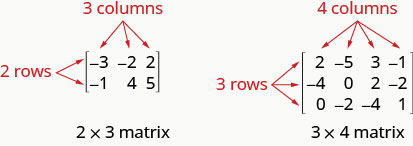
    Figure shows two matrices. The one on the left has the numbers minus 3, minus 2 and 2 in the first row and the numbers minus 1, 4 and 5 in the second row. The rows and columns are enclosed within brackets. Thus, it has 2 rows and 3 columns. It is labeled 2 cross 3 or 2 by 3 matrix. The matrix on the right is similar but with 3 rows and 4 columns. It is labeled 3 by 4 matrix.

    Each number in the matrix is called an element or entry in the matrix.

    We will use a matrix to represent a system of linear equations. We write each equation in standard form and the coefficients of the variables and the constant of each equation becomes a row in the matrix. Each column then would be the coefficients of one of the variables in the system or the constants. A vertical line replaces the equal signs. We call the resulting matrix the augmented matrix for the system of equations.

    The equations are 3x plus y equals minus 3 and 2x plus 3y equals 6. A 2 by 3 matrix is shown. The first row is 3, 1, minus 3. The second row is 2, 3, 6. The first column is labeled coefficients of x. The second column is labeled coefficients of y and the third is labeled constants.

    Notice the first column is made up of all the coefficients of x, the second column is the all the coefficients of y, and the third column is all the constants.

    Example \(\PageIndex{1}\)

    ⓐ \(\left\{ \begin{array} {l} 5x−3y=−1 \\ y=2x−2 \end{array} \right. \) ⓑ \( \left\{ \begin{array} {l} 6x−5y+2z=3 \\ 2x+y−4z=5 \\ 3x−3y+z=−1 \end{array} \right. \)

    Answer

    ⓐ The second equation is not in standard form. We rewrite the second equation in standard form.

    \[\begin{aligned} y=2x−2 \\ −2x+y=−2 \end{aligned} \nonumber\]

    We replace the second equation with its standard form. In the augmented matrix, the first equation gives us the first row and the second equation gives us the second row. The vertical line replaces the equal signs.

    The equations are 3x plus y equals minus 3 and 2x plus 3y equals 6. A 2 by 3 matrix is shown. The first row is 3, 1, minus 3. The second row is 2, 3, 6. The first column is labeled coefficients of x. The second column is labeled coefficients of y and the third is labeled constants.

    ⓑ All three equations are in standard form. In the augmented matrix the first equation gives us the first row, the second equation gives us the second row, and the third equation gives us the third row. The vertical line replaces the equal signs.

    The equations are 6x minus 5y plus 2z equals 3, 2x plus y minus 4z equals 5 and 3x minus 3y plus z equals minus 1. A 4 by 3 matrix is shown whose first row is 6, minus 5, 2, 3. Its second row is 2, 1, minus 4, 5. Its third row is 3, minus 3, 1 and minus 1. Its first three columns are labeled x, y and z respectively.

    Example \(\PageIndex{2}\)

    Write each system of linear equations as an augmented matrix:

    ⓐ \(\left\{ \begin{array} {l} 3x+8y=−3 \\ 2x=−5y−3 \end{array} \right. \) ⓑ \(\left\{ \begin{array} {l} 2x−5y+3z=8 \\ 3x−y+4z=7 \\ x+3y+2z=−3 \end{array} \right. \)

    Answer

    ⓐ \(\left[ \begin{array} {cc|c} 3 &8 &-3 \\ 2 &5 &−3 \end{array} \right] \)

    ⓑ \(\left[ \begin{array} {ccc|c} 2 &5 &-3 &8 \\ 3 &-1 &4 &7 \\ 1 &3 &2 &−3 \end{array} \right] \)

    Example \(\PageIndex{3}\)

    Write each system of linear equations as an augmented matrix:

    ⓐ \(\left\{ \begin{array} {l} 11x=−9y−5 \\ 7x+5y=−1 \end{array} \right. \) ⓑ \(\left\{ \begin{array} {l} 5x−3y+2z=−5 \\ 2x−y−z=4 \\ 3x−2y+2z=−7 \end{array} \right. \)

    Answer

    ⓐ \(\left[ \begin{array} {cc|c} 11 &9 &−5 \\ 7 &5 &−1 \end{array} \right] \)
    ⓑ \(\left[ \begin{array} {ccc|c} 5 &−3 &2 &−5 \\ 2 &−1 &−1 &4 \\ 3 &−2 &2 &−7 \end{array} \right] \)

    It is important as we solve systems of equations using matrices to be able to go back and forth between the system and the matrix. The next example asks us to take the information in the matrix and write the system of equations.

    Example \(\PageIndex{4}\)

    Write the system of equations that corresponds to the augmented matrix:

    \(\left[ \begin{array} {ccc|c} 4 &−3 &3 &−1 \\ 1 &2 &−1 &2 \\ −2 &−1 &3 &−4 \end{array} \right] \).

    Answer

    We remember that each row corresponds to an equation and that each entry is a coefficient of a variable or the constant. The vertical line replaces the equal sign. Since this matrix is a \(4\times 3\), we know it will translate into a system of three equations with three variables.

    A 3 by 4 matrix is shown. Its first row is 4, minus 3, 3, minus 1. Its second row is 1, 2, minus 1, 2. Its third row is minus 2, minus 1, 3, minus 4. The three equations are 4x minus 3y plus 3z equals minus 1, x plus 2y minus z equals 2 and minus 2x minus y plus 3z equals minus 4.

    Example \(\PageIndex{5}\)

    Write the system of equations that corresponds to the augmented matrix: \(\left[ \begin{array} {ccc|c} 1 &−1 &2 &3 \\ 2 &1 &−2 &1 \\ 4 &−1 &2 &0 \end{array} \right] \).

    Answer

    \(\left\{ \begin{array} {l} x−y+2z=3 \\ 2x+y−2z=1 \\ 4x−y+2z=0 \end{array} \right.\)

    Example \(\PageIndex{6}\)

    Write the system of equations that corresponds to the augmented matrix: \(\left[ \begin{array} {ccc|c} 1 &1 &1 &4 \\ 2 &3 &−1 &8 \\ 1 &1 &−1 &3 \end{array} \right] \).

    Answer

    \(\left\{ \begin{array} {l} x+y+z=4 \\ 2x+3y−z=8 \\ x+y−z=3 \end{array} \right.\)

    Use Row Operations on a Matrix

    Once a system of equations is in its augmented matrix form, we will perform operations on the rows that will lead us to the solution.

    To solve by elimination, it doesn’t matter which order we place the equations in the system. Similarly, in the matrix we can interchange the rows.

    When we solve by elimination, we often multiply one of the equations by a constant. Since each row represents an equation, and we can multiply each side of an equation by a constant, similarly we can multiply each entry in a row by any real number except 0.

    In elimination, we often add a multiple of one row to another row. In the matrix we can replace a row with its sum with a multiple of another row.

    These actions are called row operations and will help us use the matrix to solve a system of equations.

    ROW OPERATIONS

    In a matrix, the following operations can be performed on any row and the resulting matrix will be equivalent to the original matrix.

    1. Interchange any two rows.
    2. Multiply a row by any real number except 0.
    3. Add a nonzero multiple of one row to another row.

    Performing these operations is easy to do but all the arithmetic can result in a mistake. If we use a system to record the row operation in each step, it is much easier to go back and check our work.

    We use capital letters with subscripts to represent each row. We then show the operation to the left of the new matrix. To show interchanging a row:

    A 2 by 3 matrix is shown. Its first row, labeled R2 is 2, minus 1, 2. Its second row, labeled R1 is 5, minus 3, minus 1.

    To multiply row 2 by \(−3\):

    A 2 by 3 matrix is shown. Its first row is 5, minus 3, minus 1. Its second row is 2, minus 1, 2. An arrow point from this matrix to another one on the right. The first row of the new matrix is the same. The second row is preceded by minus 3 R2. It is minus 6, 3, minus 6.

    To multiply row 2 by \(−3\) and add it to row 1:

    A 2 by 3 matrix is shown. Its first row is 5, minus 3, minus 1. Its second row is 2, minus 1, 2. An arrow point from this matrix to another one on the right. The first row of the new matrix is preceded by minus 3 R2 plus R1. It is minus 1, 0, minus 7. The second row is 2, minus 1, 2.

    Example \(\PageIndex{7}\)

    Perform the indicated operations on the augmented matrix:

    ⓐ Interchange rows 2 and 3.

    ⓑ Multiply row 2 by 5.

    ⓒ Multiply row 3 by −2−2 and add to row 1.

    \( \left[ \begin{array} {ccc|c} 6 &−5 &2 &3 \\ 2 &1 &−4 &5 \\ 3 &−3 &1 &−1 \end{array} \right] \)

    Answer

    ⓐ We interchange rows 2 and 3.

    Two 3 by 4 matrices are shown. In the one on the left, the first row is 6, minus 5, 2, 3. The second row is 2, 1, minus 4, 5. The third row is 3, minus 3, 1, minus 1. The second matrix is similar except that rows 2 and 3 are interchanged.

    ⓑ We multiply row 2 by 5.

    Two 3 by 4 matrices are shown. In the one on the left, the first row is 6, minus 5, 2, 3. The second row is 2, 1, minus 4, 5. The third row is 3, minus 3, 1, minus 1. The second matrix is similar to the first except that row 2, preceded by 5 R2, is 10, 5, minus 20, 25.

    ⓒ We multiply row 3 by \(−2\) and add to row 1.

    In the 3 by 4 matrix, the first row is 6, minus 5, 2, 3. The second row is 2, 1, minus 4, 5. The third row is 3, minus 3, 1, minus 1. Performing the operation minus 2 R3 plus R1 on the first row, the first row becomes 6 plus minus 2 times 3, minus 5 plus minus 2 times minus 3, 2 plus minus 2 times 1 and 3 plus minus 2 times minus 1. This becomes 0, 1, 0, 5. The remaining 2 rows of the new matrix are the same.

    Example \(\PageIndex{8}\)

    Perform the indicated operations on the augmented matrix:

    ⓐ Interchange rows 1 and 3.

    ⓑ Multiply row 3 by 3.

    ⓒ Multiply row 1 by 2 and add to row 2.

    \( \left[ \begin{array} {ccc|c} 5 &−2 &-2 &-2 \\ 4 &-1 &−4 &4 \\ -2 &3 &0 &−1 \end{array} \right] \)

    Answer

    ⓐ \( \left[ \begin{array} {ccc|c} −2 &3 &0 &−2 \\ 4 &−1 &−4 &4 \\ 5 &−2 &−2 &−2 \end{array} \right] \)

    ⓑ \( \left[ \begin{array} {ccc|c}−2 &3 &0 &−2 \\ 4 &−1 &−4 &4 \\ 15 &−6 &−6 &−6 \end{array} \right] \)

    ⓒ \( \left[ \begin{array} {ccc|c} -2 &3 &0 &2 \\ 0 &5 &-4 &0  \\ 15 &-6 &-6 &-6 \end{array} \right] \)

    Example \(\PageIndex{9}\)

    Perform the indicated operations on the augmented matrix:

    ⓐ Interchange rows 1 and 2,

    ⓑ Multiply row 1 by 2,

    ⓒ Multiply row 2 by 3 and add to row 1.

    \( \left[ \begin{array} {ccc|c} 2 &−3 &−2 &−4 \\ 4 &1 &−3 &2 \\ 5 &0 &4 &−1 \end{array} \right] \)

    Answer

    ⓐ \( \left[ \begin{array} {ccc|c} 4 &1 &−3 &2 \\ 2 &−3 &−2 &−4 \\ 5 &0 &4 &−1 \end{array} \right] \)
    ⓑ \( \left[ \begin{array} {ccc|c} 8 &2 &−6 &4 \\ 2 &−3 &−2 &−4 \\ 5 &0 &4 &−1 \end{array} \right] \)
    ⓒ \( \left[ \begin{array} {ccc|c} 14 &−7 &−12 &−8 \\ 2 &−3 &−2 &−4 \\ 5 &0 &4 &−1 \end{array} \right] \)

    Now that we have practiced the row operations, we will look at an augmented matrix and figure out what operation we will use to reach a goal. This is exactly what we did when we did elimination. We decided what number to multiply a row by in order that a variable would be eliminated when we added the rows together.

    Given this system, what would you do to eliminate x?

    The two equations are x minus y equals 2 and 4x minus 8y equals 0. Multiplying the first by minus 4, we get minus 4x plus 4y equals minus 8. Adding this to the second equation we get minus 4y equals minus 8.

    This next example essentially does the same thing, but to the matrix.

    Example \(\PageIndex{10}\)

    Perform the needed row operation that will get the first entry in row 2 to be zero in the augmented matrix: \( \left[ \begin{array} {cc|c} 1 &−1 &2 \\ 4 &−8 &0 \end{array} \right] \)

    Answer

    To make the 4 a 0, we could multiply row 1 by \(−4\) and then add it to row 2.

    The 2 by 3 matrix is 1, minus 1, 2 and 4, minus 8, 0. Performing the operation minus 4R1 plus R2 on row 2, the second row of the new matrix becomes 0, minus 4, minus 8. The first row remains the same.

    Example \(\PageIndex{11}\)

    Perform the needed row operation that will get the first entry in row 2 to be zero in the augmented matrix: \( \left[ \begin{array} {cc|c} 1 &−1 &2 \\ 3 &−6 &2 \end{array} \right] \)

    Answer

    \( \left[ \begin{array} {cc|c} 1 &−1 &2 \\ 0 &−3 &−4 \end{array} \right] \)

    Example \(\PageIndex{12}\)

    Perform the needed row operation that will get the first entry in row 2 to be zero in the augmented matrix: \( \left[ \begin{array} {cc|c} 1 &−1 &3 \\ -2 &−3 &2 \end{array} \right] \)

    Answer

    \( \left[ \begin{array} {cc|c} 1 &−1 &3 \\ 0 &−5 &8 \end{array} \right] \)

    Solve Systems of Equations Using Matrices

    To solve a system of equations using matrices, we transform the augmented matrix into a matrix in row-echelon form using row operations. For a consistent and independent system of equations, its augmented matrix is in row-echelon form when to the left of the vertical line, each entry on the diagonal is a 1 and all entries below the diagonal are zeros.

    ROW-ECHELON FORM

    For a consistent and independent system of equations, its augmented matrix is in row-echelon form when to the left of the vertical line, each entry on the diagonal is a 1 and all entries below the diagonal are zeros.

    A 2 by 3 matrix is shown on the left. Its first row is 1, a, b. Its second row is 0, 1, c. An arrow points diagonally down and right, overlapping both the 1s in the matrix. A 3 by 4 matrix is shown on the right. Its first row is 1, a, b, d. Its second row is 0, 1, c, e. Its third row is 0, 0, 1, f. An arrow points diagonally down and right, overlapping all the 1s in the matrix. a, b, c, d, e, f are real numbers.

    Once we get the augmented matrix into row-echelon form, we can write the equivalent system of equations and read the value of at least one variable. We then substitute this value in another equation to continue to solve for the other variables. This process is illustrated in the next example.

    How to Solve a System of Equations Using a Matrix

    Solve the system of equations using a matrix: \(\left\{ \begin{array} {l} 3x+4y=5 \\ x+2y=1 \end{array} \right. \)

    Answer

    The equations are 3x plus 4y equals 5 and x plus 2y equals 1. Step 1. Write the augmented matrix for the system of equations. We get a 2 by 3 matrix with first row 3, 4, 5 and second row 1, 2, 1.Step 2. Using row operations get the entry in row 1, column 1 to be 1. Interchange rows R1 and R2.Step 3. Using row operations, get zeros in column 1 below the 1. Multiply row 1 by minus 3 and add it to row 2. Row 2 becomes 0, minus 2, 2.Step 4. Using row operations, get the entry in row 2, column 2 to be 1. Multiply row 2 by minus half. Row 2 becomes 0, 1, minus 1.Step 5. Continue the process until the matrix is in row-echelon form. The matrix is now in row-echelon form.Step 6. Write the corresponding system of equations. We get x plus 2y equals 1 and y equals minus 1.Step 7. Use substitution to find the remaining variables. Substitute y equals negative 1 into x plus 2y equals 1. X plus 2 times negative 1 equals 1. X minus 2 equals 1. We get x equal to 3.Step 8. Write the solution as an ordered pair or triple. Ordered pair is (3, negative 1).Step 9. Check that the solution makes the original equations true.

    Example \(\PageIndex{14}\)

    Solve the system of equations using a matrix: \(\left\{ \begin{array} {l} 2x+y=7 \\ x−2y=6 \end{array} \right. \)

    Answer

    The solution is \((4,−1)\).

    Example \(\PageIndex{15}\)

    Solve the system of equations using a matrix: \(\left\{ \begin{array} {l} 2x+y=−4 \\ x−y=−2 \end{array} \right. \)

    Answer

    The solution is \((−2,0)\).

    The steps are summarized here.

    SOLVE A SYSTEM OF EQUATIONS USING MATRICES.
    1. Write the augmented matrix for the system of equations.
    2. Using row operations get the entry in row 1, column 1 to be 1.
    3. Using row operations, get zeros in column 1 below the 1.
    4. Using row operations, get the entry in row 2, column 2 to be 1.
    5. Continue the process until the matrix is in row-echelon form.
    6. Write the corresponding system of equations.
    7. Use substitution to find the remaining variables.
    8. Write the solution as an ordered pair or triple.
    9. Check that the solution makes the original equations true.

    Here is a visual to show the order for getting the 1’s and 0’s in the proper position for row-echelon form.
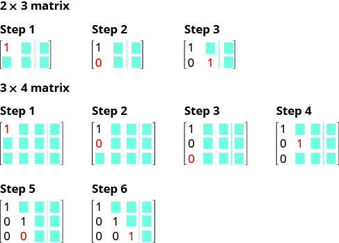
    The figure shows 3 steps for a 2 by 3 matrix and 6 steps for a 3 by 4 matrix. For the former, step 1 is to get a 1 in row 1 column 1. Step to is to get a 0 is row 2 column 1. Step 3 is to get a 1 in row 2 column 2. For a 3 by 4 matrix, step 1 is to get a 1 in row 1 column 1. Step 2 is to get a 0 in row 2 column 1. Step 3 is to get a 0 in row 3 column 1. Step 4 is to get a 1 in row 2 column 2. Step 5 is to get a 0 in row 3 column 2. Step 6 is to get a 1 in row 3 column 3.

    We use the same procedure when the system of equations has three equations.

    Example \(\PageIndex{16}\)

    Solve the system of equations using a matrix: \(\left\{ \begin{array} {l} 3x+8y+2z=−5 \\ 2x+5y−3z=0 \\ x+2y−2z=−1 \end{array} \right. \)

    Answer
      .
    Write the augmented matrix for the equations. .
    Interchange row 1 and 3 to get the entry in
    row 1, column 1 to be 1.
    .
    Using row operations, get zeros in column 1 below the 1. .
      .
    The entry in row 2, column 2 is now 1.  
    Continue the process until the matrix
    is in row-echelon form.
    .
      .
    The matrix is now in row-echelon form. .
    Write the corresponding system of equations. .
    Use substitution to find the remaining variables. .
      .
    .
    Write the solution as an ordered pair or triple. .
    Check that the solution makes the original equations true. We leave the check for you.
    Example \(\PageIndex{17}\)

    Solve the system of equations using a matrix: \(\left\{ \begin{array} {l} 2x−5y+3z=8 \\ 3x−y+4z=7 \\ x+3y+2z=−3 \end{array} \right. \)

    Answer

    \((6,−1,−3)\)

    Example \(\PageIndex{18}\)

    Solve the system of equations using a matrix: \(\left\{ \begin{array} {l} −3x+y+z=−4 \\ −x+2y−2z=1 \\ 2x−y−z=−1 \end{array} \right. \)

    Answer

    \((5,7,4)\)

    So far our work with matrices has only been with systems that are consistent and independent, which means they have exactly one solution. Let’s now look at what happens when we use a matrix for a dependent or inconsistent system.

    Example \(\PageIndex{19}\)

    Solve the system of equations using a matrix: \(\left\{ \begin{array} {l} x+y+3z=0 \\ x+3y+5z=0 \\ 2x+4z=1 \end{array} \right. \)

    Answer
      .
    Write the augmented matrix for the equations. .
    The entry in row 1, column 1 is 1.  
    Using row operations, get zeros in column 1 below the 1. .
      .
    Continue the process until the matrix is in row-echelon form. .
    Multiply row 2 by 2 and add it to row 3. .
    At this point, we have all zeros on the left of row 3.  
    Write the corresponding system of equations. .
    Since \(0 \neq 1 \) we have a false statement. Just as when we solved a system using other methods, this tells us we have an inconsistent system. There is no solution.
    Example \(\PageIndex{20}\)

    Solve the system of equations using a matrix: \(\left\{ \begin{array} {l} x−2y+2z=1 \\ −2x+y−z=2 \\ x−y+z=5 \end{array} \right. \)

    Answer

    no solution

    Example \(\PageIndex{21}\)

    Solve the system of equations using a matrix: \(\left\{ \begin{array} {l} 3x+4y−3z=−2 \\ −2x+3y−z=−1 \\ 2x+y−2z=6 \end{array} \right. \)

    Answer

    no solution

    The last system was inconsistent and so had no solutions. The next example is dependent and has infinitely many solutions.

    Example \(\PageIndex{22}\)

    Solve the system of equations using a matrix: \(\left\{ \begin{array} {l} x−2y+3z=1 \\ x+y−3z=7 \\ 3x−4y+5z=7 \end{array} \right. \)

    Answer
      .
    Write the augmented matrix for the equations. .
    The entry in row 1, column 1 is 1.  
    Using row operations, get zeros in column 1 below the 1. .
      .
    Continue the process until the matrix is in row-echelon form. .
    Multiply row 2 by \(−2\) and add it to row 3. .
    At this point, we have all zeros in the bottom row.  
    Write the corresponding system of equations. .
    Since \(0=0\) we have a true statement. Just as when we solved by substitution, this tells us we have a dependent system. There are infinitely many solutions.
    Solve for y in terms of z in the second equation. .
    Solve the first equation for x in terms of z. .
    Substitute \(y=2z+2\). .
    Simplify. .
    Simplify. .
    Simplify. .
    The system has infinitely many solutions \((x,y,z)\), where \(x=z+5;\space y=2z+2;\space z\) is any real number.
    Example \(\PageIndex{23}\)

    Solve the system of equations using a matrix: \(\left\{ \begin{array} {l} x+y−z=0 \\ 2x+4y−2z=6 \\ 3x+6y−3z=9 \end{array} \right. \)

    Answer

    infinitely many solutions \((x,y,z)\), where \(x=z−3;\space y=3;\space z\) is any real number.

    Example \(\PageIndex{24}\)

    Solve the system of equations using a matrix: \(\left\{ \begin{array} {l} x−y−z=1 \\ −x+2y−3z=−4 \\ 3x−2y−7z=0 \end{array} \right. \)

    Answer

    infinitely many solutions \((x,y,z)\), where \(x=5z−2;\space y=4z−3;\space z\) is any real number.

    Access this online resource for additional instruction and practice with Gaussian Elimination.

    • Gaussian Elimination

    Key Concepts

    • Matrix: A matrix is a rectangular array of numbers arranged in rows and columns. A matrix with m rows and n columns has order \(m\times n\). The matrix on the left below has 2 rows and 3 columns and so it has order \(2\times 3\). We say it is a 2 by 3 matrix.
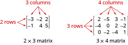
      Figure shows two matrices. The one on the left has the numbers minus 3, minus 2 and 2 in the first row and the numbers minus 1, 4 and 5 in the second row. The rows and columns are enclosed within brackets. Thus, it has 2 rows and 3 columns. It is labeled 2 cross 3 or 2 by 3 matrix. The matrix on the right is similar but with 3 rows and 4 columns. It is labeled 3 by 4 matrix.
      Each number in the matrix is called an element or entry in the matrix.
    • Row Operations: In a matrix, the following operations can be performed on any row and the resulting matrix will be equivalent to the original matrix.
      • Interchange any two rows
      • Multiply a row by any real number except 0
      • Add a nonzero multiple of one row to another row
    • Row-Echelon Form: For a consistent and independent system of equations, its augmented matrix is in row-echelon form when to the left of the vertical line, each entry on the diagonal is a 1 and all entries below the diagonal are zeros.
      Figure shows two matrices. The one on the left has the numbers minus 3, minus 2 and 2 in the first row and the numbers minus 1, 4 and 5 in the second row. The rows and columns are enclosed within brackets. Thus, it has 2 rows and 3 columns. It is labeled 2 cross 3 or 2 by 3 matrix. The matrix on the right is similar but with 3 rows and 4 columns. It is labeled 3 by 4 matrix.
    • How to solve a system of equations using matrices.
      1. Write the augmented matrix for the system of equations.
      2. Using row operations get the entry in row 1, column 1 to be 1.
      3. Using row operations, get zeros in column 1 below the 1.
      4. Using row operations, get the entry in row 2, column 2 to be 1.
      5. Continue the process until the matrix is in row-echelon form.
      6. Write the corresponding system of equations.
      7. Use substitution to find the remaining variables.
      8. Write the solution as an ordered pair or triple.
      9. Check that the solution makes the original equations true.

    Glossary

    matrix
    A matrix is a rectangular array of numbers arranged in rows and columns.
    row-echelon form
    A matrix is in row-echelon form when to the left of the vertical line, each entry on the diagonal is a 1 and all entries below the diagonal are zeros.

    This page titled 3.6: Solve Systems of Equations Using Matrices is shared under a CC BY license and was authored, remixed, and/or curated by OpenStax.

    • Was this article helpful?