Mathematics LibreTexts

3.8: Chapter 7 Review Exercises

  • Page ID
    130092
    • Gilbert Strang & Edwin “Jed” Herman
    • OpenStax

    \( \newcommand{\vecs}[1]{\overset { \scriptstyle \rightharpoonup} {\mathbf{#1}} } \)

    \( \newcommand{\vecd}[1]{\overset{-\!-\!\rightharpoonup}{\vphantom{a}\smash {#1}}} \)

    \( \newcommand{\id}{\mathrm{id}}\) \( \newcommand{\Span}{\mathrm{span}}\)

    ( \newcommand{\kernel}{\mathrm{null}\,}\) \( \newcommand{\range}{\mathrm{range}\,}\)

    \( \newcommand{\RealPart}{\mathrm{Re}}\) \( \newcommand{\ImaginaryPart}{\mathrm{Im}}\)

    \( \newcommand{\Argument}{\mathrm{Arg}}\) \( \newcommand{\norm}[1]{\| #1 \|}\)

    \( \newcommand{\inner}[2]{\langle #1, #2 \rangle}\)

    \( \newcommand{\Span}{\mathrm{span}}\)

    \( \newcommand{\id}{\mathrm{id}}\)

    \( \newcommand{\Span}{\mathrm{span}}\)

    \( \newcommand{\kernel}{\mathrm{null}\,}\)

    \( \newcommand{\range}{\mathrm{range}\,}\)

    \( \newcommand{\RealPart}{\mathrm{Re}}\)

    \( \newcommand{\ImaginaryPart}{\mathrm{Im}}\)

    \( \newcommand{\Argument}{\mathrm{Arg}}\)

    \( \newcommand{\norm}[1]{\| #1 \|}\)

    \( \newcommand{\inner}[2]{\langle #1, #2 \rangle}\)

    \( \newcommand{\Span}{\mathrm{span}}\) \( \newcommand{\AA}{\unicode[.8,0]{x212B}}\)

    \( \newcommand{\vectorA}[1]{\vec{#1}}      % arrow\)

    \( \newcommand{\vectorAt}[1]{\vec{\text{#1}}}      % arrow\)

    \( \newcommand{\vectorB}[1]{\overset { \scriptstyle \rightharpoonup} {\mathbf{#1}} } \)

    \( \newcommand{\vectorC}[1]{\textbf{#1}} \)

    \( \newcommand{\vectorD}[1]{\overrightarrow{#1}} \)

    \( \newcommand{\vectorDt}[1]{\overrightarrow{\text{#1}}} \)

    \( \newcommand{\vectE}[1]{\overset{-\!-\!\rightharpoonup}{\vphantom{a}\smash{\mathbf {#1}}}} \)

    \( \newcommand{\vecs}[1]{\overset { \scriptstyle \rightharpoonup} {\mathbf{#1}} } \)

    \( \newcommand{\vecd}[1]{\overset{-\!-\!\rightharpoonup}{\vphantom{a}\smash {#1}}} \)

    \(\newcommand{\avec}{\mathbf a}\) \(\newcommand{\bvec}{\mathbf b}\) \(\newcommand{\cvec}{\mathbf c}\) \(\newcommand{\dvec}{\mathbf d}\) \(\newcommand{\dtil}{\widetilde{\mathbf d}}\) \(\newcommand{\evec}{\mathbf e}\) \(\newcommand{\fvec}{\mathbf f}\) \(\newcommand{\nvec}{\mathbf n}\) \(\newcommand{\pvec}{\mathbf p}\) \(\newcommand{\qvec}{\mathbf q}\) \(\newcommand{\svec}{\mathbf s}\) \(\newcommand{\tvec}{\mathbf t}\) \(\newcommand{\uvec}{\mathbf u}\) \(\newcommand{\vvec}{\mathbf v}\) \(\newcommand{\wvec}{\mathbf w}\) \(\newcommand{\xvec}{\mathbf x}\) \(\newcommand{\yvec}{\mathbf y}\) \(\newcommand{\zvec}{\mathbf z}\) \(\newcommand{\rvec}{\mathbf r}\) \(\newcommand{\mvec}{\mathbf m}\) \(\newcommand{\zerovec}{\mathbf 0}\) \(\newcommand{\onevec}{\mathbf 1}\) \(\newcommand{\real}{\mathbb R}\) \(\newcommand{\twovec}[2]{\left[\begin{array}{r}#1 \\ #2 \end{array}\right]}\) \(\newcommand{\ctwovec}[2]{\left[\begin{array}{c}#1 \\ #2 \end{array}\right]}\) \(\newcommand{\threevec}[3]{\left[\begin{array}{r}#1 \\ #2 \\ #3 \end{array}\right]}\) \(\newcommand{\cthreevec}[3]{\left[\begin{array}{c}#1 \\ #2 \\ #3 \end{array}\right]}\) \(\newcommand{\fourvec}[4]{\left[\begin{array}{r}#1 \\ #2 \\ #3 \\ #4 \end{array}\right]}\) \(\newcommand{\cfourvec}[4]{\left[\begin{array}{c}#1 \\ #2 \\ #3 \\ #4 \end{array}\right]}\) \(\newcommand{\fivevec}[5]{\left[\begin{array}{r}#1 \\ #2 \\ #3 \\ #4 \\ #5 \\ \end{array}\right]}\) \(\newcommand{\cfivevec}[5]{\left[\begin{array}{c}#1 \\ #2 \\ #3 \\ #4 \\ #5 \\ \end{array}\right]}\) \(\newcommand{\mattwo}[4]{\left[\begin{array}{rr}#1 \amp #2 \\ #3 \amp #4 \\ \end{array}\right]}\) \(\newcommand{\laspan}[1]{\text{Span}\{#1\}}\) \(\newcommand{\bcal}{\cal B}\) \(\newcommand{\ccal}{\cal C}\) \(\newcommand{\scal}{\cal S}\) \(\newcommand{\wcal}{\cal W}\) \(\newcommand{\ecal}{\cal E}\) \(\newcommand{\coords}[2]{\left\{#1\right\}_{#2}}\) \(\newcommand{\gray}[1]{\color{gray}{#1}}\) \(\newcommand{\lgray}[1]{\color{lightgray}{#1}}\) \(\newcommand{\rank}{\operatorname{rank}}\) \(\newcommand{\row}{\text{Row}}\) \(\newcommand{\col}{\text{Col}}\) \(\renewcommand{\row}{\text{Row}}\) \(\newcommand{\nul}{\text{Nul}}\) \(\newcommand{\var}{\text{Var}}\) \(\newcommand{\corr}{\text{corr}}\) \(\newcommand{\len}[1]{\left|#1\right|}\) \(\newcommand{\bbar}{\overline{\bvec}}\) \(\newcommand{\bhat}{\widehat{\bvec}}\) \(\newcommand{\bperp}{\bvec^\perp}\) \(\newcommand{\xhat}{\widehat{\xvec}}\) \(\newcommand{\vhat}{\widehat{\vvec}}\) \(\newcommand{\uhat}{\widehat{\uvec}}\) \(\newcommand{\what}{\widehat{\wvec}}\) \(\newcommand{\Sighat}{\widehat{\Sigma}}\) \(\newcommand{\lt}{<}\) \(\newcommand{\gt}{>}\) \(\newcommand{\amp}{&}\) \(\definecolor{fillinmathshade}{gray}{0.9}\)

    In exercises 1 - 4, determine whether the statement is true or false. Justify your answer with a proof or a counterexample.

    1) \(\displaystyle ∫e^x\sin(x)\,dx\) cannot be integrated by parts.

    2) \(\displaystyle ∫\frac{1}{x^4+1}\,dx\) cannot be integrated using partial fractions.

    Answer
    False

    3) In numerical integration, increasing the number of points decreases the error.

    4) Integration by parts can always yield the integral.

    Answer
    False

    In exercises 5 - 10, evaluate the integral using the specified method.

    5) \(\displaystyle ∫x^2\sin(4x)\,dx,\) using integration by parts

    6) \(\displaystyle ∫\frac{1}{x^2\sqrt{x^2+16}}\,dx,\) using trigonometric substitution

    Answer
    \(\displaystyle ∫\frac{1}{x^2\sqrt{x^2+16}}\,dx = −\frac{\sqrt{x^2+16}}{16x}+C\)

    7) \(\displaystyle ∫\sqrt{x}\ln x\,dx,\) using integration by parts

    8) \(\displaystyle ∫\frac{3x}{x^3+2x^2−5x−6}\,dx,\) using partial fractions

    Answer
    \(\displaystyle ∫\frac{3x}{x^3+2x^2−5x−6}\,dx = \frac{1}{10}\big(4\ln|2−x|+5\ln|x+1|−9\ln|x+3|\big)+C\)

    9) \(\displaystyle ∫\frac{x^5}{(4x^2+4)^{5/2}}\,dx,\) using trigonometric substitution

    10) \(\displaystyle ∫\frac{\sqrt{4−\sin^2(x)}}{\sin^2(x)}\cos(x)\,dx,\) using a table of integrals or a CAS

    Answer
    \(\displaystyle ∫\frac{\sqrt{4−\sin^2(x)}}{\sin^2(x)}\cos(x)\,dx = −\frac{\sqrt{4−\sin^2(x)}}{\sin(x)}−\frac{x}{2}+C\)

    In exercises 11 - 15, integrate using whatever method you choose.

    11) \(\displaystyle ∫\sin^2 x\cos^2 x\,dx\)

    12) \(\displaystyle ∫x^3\sqrt{x^2+2}\,dx\)

    Answer
    \(\displaystyle ∫x^3\sqrt{x^2+2}\,dx = \frac{1}{15}(x^2+2)^{3/2}(3x^2−4)+C\)

    13) \(\displaystyle ∫\frac{3x^2+1}{x^4−2x^3−x^2+2x}\,dx\)

    14) \(\displaystyle ∫\frac{1}{x^4+4}\,dx\)

    Answer
    \(\displaystyle ∫\frac{1}{x^4+4}\,dx = \frac{1}{16}\ln(\frac{x^2+2x+2}{x^2−2x+2})−\frac{1}{8}\tan^{−1}(1−x)+\frac{1}{8}\tan^{−1}(x+1)+C\)

    15) \(\displaystyle ∫\frac{\sqrt{3+16x^4}}{x^4}\,dx\)

    In exercises 16 - 18, approximate the integrals using the midpoint rule, trapezoidal rule, and Simpson’s rule using four subintervals, rounding to three decimals.

    16) [T] \(\displaystyle ∫^2_1\sqrt{x^5+2}\,dx\)

    Answer
    \(M_4=3.312,\)
    \(T_4=3.354,\)
    \(S_4=3.326\)

    17) [T] \(\displaystyle ∫^{\sqrt{π}}_0e^{−\sin(x^2)}\,dx\)

    18) [T] \(\displaystyle ∫^4_1\frac{\ln(1/x)}{x}\,dx\)

    Answer
    \(M_4=−0.982,\)
    \(T_4=−0.917,\)
    \(S_4=−0.952\)

    In exercises 19 - 20, evaluate the integrals, if possible.

    19) \(\displaystyle ∫^∞_1\frac{1}{x^n}\,dx,\) for what values of \(n\) does this integral converge or diverge?

    20) \(\displaystyle ∫^∞_1\frac{e^{−x}}{x}\,dx\)

    Answer
    approximately 0.2194

    In exercises 21 - 22, consider the gamma function given by \(\displaystyle Γ(a)=∫^∞_0e^{−y}y^{a−1}\,dy.\)

    21) Show that \(\displaystyle Γ(a)=(a−1)Γ(a−1).\)

    22) Extend to show that \(\displaystyle Γ(a)=(a−1)!,\) assuming \(a\) is a positive integer.

    The fastest car in the world, the Bugati Veyron, can reach a top speed of 408 km/h. The graph represents its velocity.
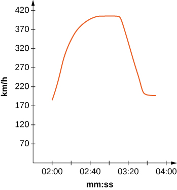
    This figure has a graph in the first quadrant. It increases to where x is approximately 03:00 mm:ss and then drops off steep. The maximum height of the graph, here the drop occurs is approximately 420 km/h.

    23) [T] Use the graph to estimate the velocity every 20 sec and fit to a graph of the form \(v(t)=ae^{bx}\sin(cx)+d.\) (Hint: Consider the time units.)

    24) [T] Using your function from the previous problem, find exactly how far the Bugati Veyron traveled in the 1 min 40 sec included in the graph.

    Answer
    Answers may vary. Ex: \(9.405\) km

    This page titled 3.8: Chapter 7 Review Exercises is shared under a CC BY-NC-SA 4.0 license and was authored, remixed, and/or curated by Gilbert Strang & Edwin “Jed” Herman (OpenStax) via source content that was edited to the style and standards of the LibreTexts platform.