
Creating Dynamic Figures with CalcPlot3D
- Page ID
- 75457

\( \newcommand{\vecs}[1]{\overset { \scriptstyle \rightharpoonup} {\mathbf{#1}} } \)
\( \newcommand{\vecd}[1]{\overset{-\!-\!\rightharpoonup}{\vphantom{a}\smash {#1}}} \)
\( \newcommand{\dsum}{\displaystyle\sum\limits} \)
\( \newcommand{\dint}{\displaystyle\int\limits} \)
\( \newcommand{\dlim}{\displaystyle\lim\limits} \)
\( \newcommand{\id}{\mathrm{id}}\) \( \newcommand{\Span}{\mathrm{span}}\)
( \newcommand{\kernel}{\mathrm{null}\,}\) \( \newcommand{\range}{\mathrm{range}\,}\)
\( \newcommand{\RealPart}{\mathrm{Re}}\) \( \newcommand{\ImaginaryPart}{\mathrm{Im}}\)
\( \newcommand{\Argument}{\mathrm{Arg}}\) \( \newcommand{\norm}[1]{\| #1 \|}\)
\( \newcommand{\inner}[2]{\langle #1, #2 \rangle}\)
\( \newcommand{\Span}{\mathrm{span}}\)
\( \newcommand{\id}{\mathrm{id}}\)
\( \newcommand{\Span}{\mathrm{span}}\)
\( \newcommand{\kernel}{\mathrm{null}\,}\)
\( \newcommand{\range}{\mathrm{range}\,}\)
\( \newcommand{\RealPart}{\mathrm{Re}}\)
\( \newcommand{\ImaginaryPart}{\mathrm{Im}}\)
\( \newcommand{\Argument}{\mathrm{Arg}}\)
\( \newcommand{\norm}[1]{\| #1 \|}\)
\( \newcommand{\inner}[2]{\langle #1, #2 \rangle}\)
\( \newcommand{\Span}{\mathrm{span}}\) \( \newcommand{\AA}{\unicode[.8,0]{x212B}}\)
\( \newcommand{\vectorA}[1]{\vec{#1}} % arrow\)
\( \newcommand{\vectorAt}[1]{\vec{\text{#1}}} % arrow\)
\( \newcommand{\vectorB}[1]{\overset { \scriptstyle \rightharpoonup} {\mathbf{#1}} } \)
\( \newcommand{\vectorC}[1]{\textbf{#1}} \)
\( \newcommand{\vectorD}[1]{\overrightarrow{#1}} \)
\( \newcommand{\vectorDt}[1]{\overrightarrow{\text{#1}}} \)
\( \newcommand{\vectE}[1]{\overset{-\!-\!\rightharpoonup}{\vphantom{a}\smash{\mathbf {#1}}}} \)
\( \newcommand{\vecs}[1]{\overset { \scriptstyle \rightharpoonup} {\mathbf{#1}} } \)
\(\newcommand{\longvect}{\overrightarrow}\)
\( \newcommand{\vecd}[1]{\overset{-\!-\!\rightharpoonup}{\vphantom{a}\smash {#1}}} \)
\(\newcommand{\avec}{\mathbf a}\) \(\newcommand{\bvec}{\mathbf b}\) \(\newcommand{\cvec}{\mathbf c}\) \(\newcommand{\dvec}{\mathbf d}\) \(\newcommand{\dtil}{\widetilde{\mathbf d}}\) \(\newcommand{\evec}{\mathbf e}\) \(\newcommand{\fvec}{\mathbf f}\) \(\newcommand{\nvec}{\mathbf n}\) \(\newcommand{\pvec}{\mathbf p}\) \(\newcommand{\qvec}{\mathbf q}\) \(\newcommand{\svec}{\mathbf s}\) \(\newcommand{\tvec}{\mathbf t}\) \(\newcommand{\uvec}{\mathbf u}\) \(\newcommand{\vvec}{\mathbf v}\) \(\newcommand{\wvec}{\mathbf w}\) \(\newcommand{\xvec}{\mathbf x}\) \(\newcommand{\yvec}{\mathbf y}\) \(\newcommand{\zvec}{\mathbf z}\) \(\newcommand{\rvec}{\mathbf r}\) \(\newcommand{\mvec}{\mathbf m}\) \(\newcommand{\zerovec}{\mathbf 0}\) \(\newcommand{\onevec}{\mathbf 1}\) \(\newcommand{\real}{\mathbb R}\) \(\newcommand{\twovec}[2]{\left[\begin{array}{r}#1 \\ #2 \end{array}\right]}\) \(\newcommand{\ctwovec}[2]{\left[\begin{array}{c}#1 \\ #2 \end{array}\right]}\) \(\newcommand{\threevec}[3]{\left[\begin{array}{r}#1 \\ #2 \\ #3 \end{array}\right]}\) \(\newcommand{\cthreevec}[3]{\left[\begin{array}{c}#1 \\ #2 \\ #3 \end{array}\right]}\) \(\newcommand{\fourvec}[4]{\left[\begin{array}{r}#1 \\ #2 \\ #3 \\ #4 \end{array}\right]}\) \(\newcommand{\cfourvec}[4]{\left[\begin{array}{c}#1 \\ #2 \\ #3 \\ #4 \end{array}\right]}\) \(\newcommand{\fivevec}[5]{\left[\begin{array}{r}#1 \\ #2 \\ #3 \\ #4 \\ #5 \\ \end{array}\right]}\) \(\newcommand{\cfivevec}[5]{\left[\begin{array}{c}#1 \\ #2 \\ #3 \\ #4 \\ #5 \\ \end{array}\right]}\) \(\newcommand{\mattwo}[4]{\left[\begin{array}{rr}#1 \amp #2 \\ #3 \amp #4 \\ \end{array}\right]}\) \(\newcommand{\laspan}[1]{\text{Span}\{#1\}}\) \(\newcommand{\bcal}{\cal B}\) \(\newcommand{\ccal}{\cal C}\) \(\newcommand{\scal}{\cal S}\) \(\newcommand{\wcal}{\cal W}\) \(\newcommand{\ecal}{\cal E}\) \(\newcommand{\coords}[2]{\left\{#1\right\}_{#2}}\) \(\newcommand{\gray}[1]{\color{gray}{#1}}\) \(\newcommand{\lgray}[1]{\color{lightgray}{#1}}\) \(\newcommand{\rank}{\operatorname{rank}}\) \(\newcommand{\row}{\text{Row}}\) \(\newcommand{\col}{\text{Col}}\) \(\renewcommand{\row}{\text{Row}}\) \(\newcommand{\nul}{\text{Nul}}\) \(\newcommand{\var}{\text{Var}}\) \(\newcommand{\corr}{\text{corr}}\) \(\newcommand{\len}[1]{\left|#1\right|}\) \(\newcommand{\bbar}{\overline{\bvec}}\) \(\newcommand{\bhat}{\widehat{\bvec}}\) \(\newcommand{\bperp}{\bvec^\perp}\) \(\newcommand{\xhat}{\widehat{\xvec}}\) \(\newcommand{\vhat}{\widehat{\vvec}}\) \(\newcommand{\uhat}{\widehat{\uvec}}\) \(\newcommand{\what}{\widehat{\wvec}}\) \(\newcommand{\Sighat}{\widehat{\Sigma}}\) \(\newcommand{\lt}{<}\) \(\newcommand{\gt}{>}\) \(\newcommand{\amp}{&}\) \(\definecolor{fillinmathshade}{gray}{0.9}\)Overview
CalcPlot3D is a free online visualization tool originally developed to help students learn concepts in multivariable calculus, but now offering visual tools that can be useful in many STEM courses. Using CalcPlot3D, authors of LibreTexts can create and insert dynamic figures of two basic types:
- Rotatable 3D dynamic plots with no external controls
- 2D and 3D dynamic plots with scrollbars and some other controls
See examples in Figures \(\PageIndex{1}\) - \(\PageIndex{3}\) below.
As you can see in these examples, both types of dynamic figures can be helpful. Sometimes a rotatable 3D plot is all that is needed. But in other situations, adjusting various parameters with scrollbars, textboxes, and checkboxes can greatly aid student understanding.
Inserting Pre-made CalcPlot3D Dynamic Figures from the Learning Objects Library
This is the easiest way to get started using CalcPlot3D dynamic figures, since it only requires you to browse the Learning Objects library, find a dynamic figure you'd like to use, and then to use the Content reuse option on the Elements menu to insert it into your LibreTexts page. But this approach does not allow you to adjust the parameters of the interactive figures. You get exactly what's there already. So you may wish to continue to creating your own dynamic figures using CalcPlot3D.
Steps to inserting an existing CalcPlot3D dynamic figure into a LibreTexts page:
- Browse the CalcPlot3D Interactives library (this link is for the one on the LibreTexts Math Library) and find a dynamic figure you'd like to use in your custom page.
- Select Elements > Content reuse from the edit menu. Then click the + in front of Home. You should now see the Learning Objects library. Click on the + in front of Learning Objects and navaigate to find the dynamic figure you found in the previous step.
You should get an object that looks like the following:

And renders as:
If you would like to place a CalcPlot3D dynamic figure from the Learning Objects library in a figure, there is a template for that.
Select Elements > Templates and choose Template:AddFigureCalcPlot3DReuse (available on the LibreTexts Math Library). It will generate the following placeholder:

You can then follow the instructions at the top of the placeholder to right-click on the content reuse object, select Edit content reuse, and adjust the selection to the CalcPlot3D dynamic figure you want to use. Update the figure caption and remove the instructional text at the top of the figure and you'll be all set!
See examples in the Overview section at the top of this page.
Inserting Pre-made CalcPlot3D Figures from a Different LibreTexts Library
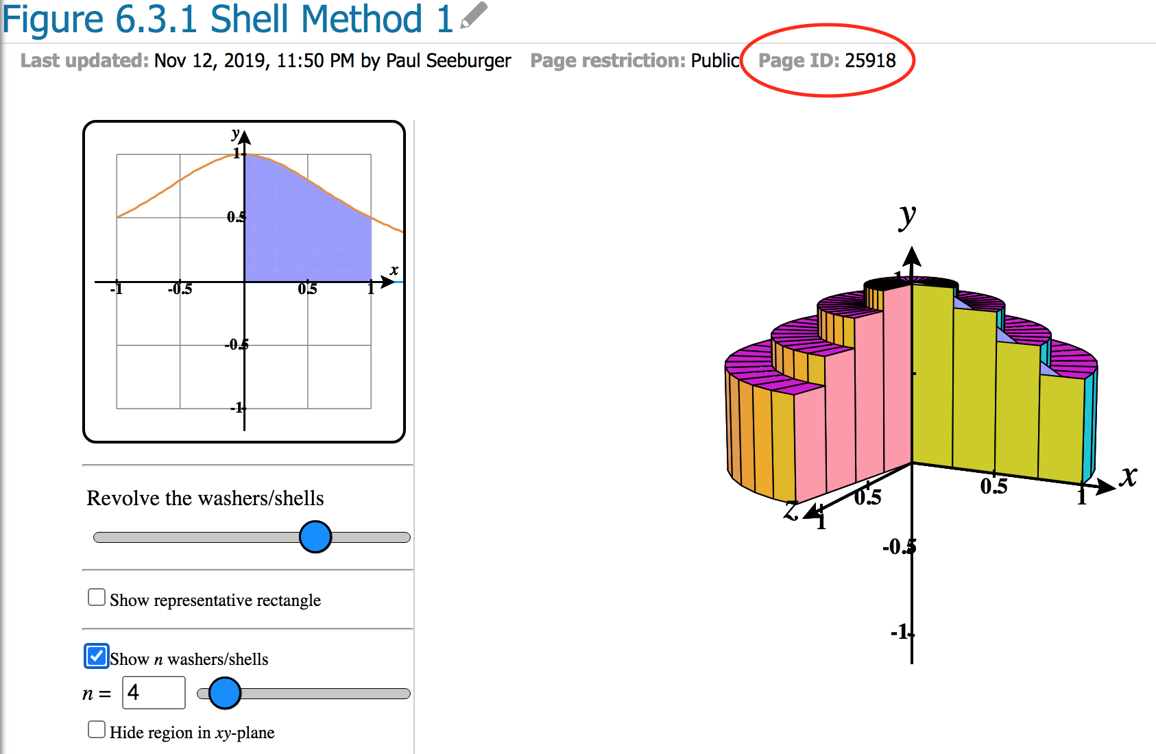
If you decide you'd like to insert a CalcPlot3D dynamic figure from a LibreTexts library other than the one in which you are building your custom text, this can be accomplished using a Cross-Library Reference, the library subject area, and the Page ID number for the CalcPlot3D dynamic figure you have selected.
Say we wish to insert the following figure from the LibreTexts Math Library on a page in another LibreTexts library (say Chemistry or Physics).
We would need to create a new page, name it, and then save it (before editing it) to set it up with the correct codes. Then we would edit the page again and click on the </> HTML button on the right end of the editing toolbar. Enter the following code.
<p class="mt-script-comment">Cross Library Transclusion</p>

<pre class="script">
template('CrossTransclude/Web',{'Library':'math','PageID':25918});</pre>
Saving your page should reveal the CalcPlot3D dynamic figure you wanted. This code could also be placed inside a LibreTexts page with other text and figures, or you could set up a collection of figures each in their own page that you could easily place in other pages using the Content Reuse approach described above.
This Cross Library Transclusion code can be used to insert any content from another library into your custom LibreTexts.
Creating your own CalcPlot3D Dynamic Figures using CalcPlot3D (without controls)
In this section, we'll discuss how to generate your own CalcPlot3D dynamic figures using the CalcPlot3D app. As stated above, there are two types, a basic rotatable 3D plot with no controls, and a 2D or 3D plot with controls. Since the first type is easiest to implement, we'll start there and then cover the second variety in the section titled Creating your own Dynamic Figures using CalcPlot3D (with controls) below.
- Open CalcPlot3D and work out the figure you wish to include in your LibreTexts page. See the CalcPlot3D Help Manual for assistance with this.
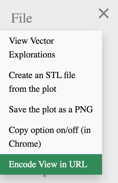
- Once you have the 3D plot as you want it to appear in the dynamic figure (including the initial orientation), click on the menu icon (☰) in the upper-left corner of the app, select File and then Encode View in URL. See Figure \(\PageIndex{7}\) below.
The page will reload with the new URL that will include a script that specifies the initial view. It should match the view you had set up in step 1. - Copy the entire query string following the question mark in the URL to the system clipboard. Ctrl-c (cmd-c on a Mac) will help you do this.
- Use this query string to paste into the HTML code shown below in either the section titled Creating Sharable CalcPlot3D Interactives in LibreTexts or the section titled Using Template:AddFigureCalcPlot3DNew to Insert your New CalcPlot3D Dynamic Figures (without controls). Note that the second approach is easier for beginners, but there are some advantages to organizing your CalcPlot3D dynamic figures in a repository folder (see the next section).
Creating Sharable CalcPlot3D Interactive Figures in LibreTexts
There is at least one advantage to creating standalone CalcPlot3D dynamic figure pages in your own repository folder (a "Book" in your Campus Hub or Sandbox). It makes your interactive figures much easier to share with others. All they need to do is follow the instructions above to use content reuse to insert your figures into their pages.
It also allows you to easily update the code for all your figures in one place. And if you happen to want a particular figure in multiple places in your LibreTexts, it's a great way to use transclusion to minimize the code you have to maintain moving forward.
This was the approach used to create the library of CalcPlot3D Interactive Figures in the Learning Objects library.
Since the typical user does not have permissions to add new objects there, we will cover how you can create your own repository of CalcPlot3D Interactive Figures. Initially you may practice this process in your Sandbox, but eventually you'll want to move your repository to your Campus Hub, once you have access to it. Note that all links should update when you decide to move this folder. You may wish to make the folder containing these files semi-private using the Permissions menu option on the Options menu for the folder.
The first step in this process is to get a copy of one of the existing CalcPlot3D figures (without controls) into this folder. You have two options to do this for the first time.
- You can use the Remixer, possibly even using it to create the new "book" which will serve as a repository for your personally created CalcPlot3D dynamic figures, or
- You can create a new Book in your Sandbox (or Campus Hub), naming it CalcPlot3D Repository (or similar), and then create a new page in this book. Then use Elements > Content reuse to import an existing CalcPlot3D figure into that page. Bee sure there is nothing else in the page.
Once you have a transcluded copy of a CalcPlot3D figure, you will need to fork the page using the Forker option on the Options menu for the page (or the fork symbol to the right of the page title, if you used the Remixer). This should give you a full copy of a CalcPlot3D dynamic figure of your own to edit.
Once you have used either of these approaches, you should have a linked/transcluded copy of a CalcPlot3D dynamic figure in your repository folder. To create additional CalcPlot3D figures, you can just copy this one, giving it a new name!
From this new forked page, click the Edit button on the login bar. Note that the CalcPlot3D figure will still appear in rendered form in Visual edit mode. Click the </> HTML button in the upper-right corner of the edit window to change to HTML mode.
Replace the code shown highlighted in blue in Figure \(\PageIndex{8}\) with the query string you formed in Step 3 in the previous section. Note that depending on the figure you chose for this placeholder, the code may be longer or shorter than what is shown in this figure.

Clicking of the Visual button to toggle back to view the WYSIWYG mode of the editor will actually let you see how the CalcPlot3D figure looks before you save it. If you need to adjust anything in the code, you can switch back to adjust it using the </> HTML button again. One of the most common options that you may wish to adjust is the zoom option, located about 4 script commands from the end of the query string. Decreasing the decimal number will make the 3D plot smaller. Increasing it will make the 3D plot larger.
You can actually adjust any of the options in the string, many of which are fairly intuitive. But these could also be adjusted using CalcPlot3D and updating the URL query string.
Note that when you create CalcPlot3D figures with this approach, it is very helpful to add a static image of the figure to the page holding the code for it. This makes the figures much easier to quickly browse in your repository, although it takes an extra step on your part.
Adding a Static Image to your Sharable CalcPlot3D Figure
Once the figure looks as you want it to look, take a screen snip of the figure using a tool like Snip & Sketch on Windows (or Shift-Cmd-4) to create and save an static image to serve as the thumbnail for this figure. Then open the Page Settings at the top of the page by clicking anywhere on this gray bar.
If the Article Type is not Book or Unit or Chapter, change it to one of these. This will allow the Thumbnail option to be shown. Once you have changed the Article Type, reload the page.
Next hover over the thumbnail image (it may be blank) in the upper-left corner and click on the pencil you should see there. This should allow you to load your saved thumbnail image and you will be all set!
Inserting your own CalcPlot3D Dynamic Figures in LibreTexts Pages
Next we will want to insert our new dynamic figure into a LibreTexts page. There are two basic ways to do this. We can either use Content reuse or the template, Template:AddFigureCalcPlot3DReuse to insert the new sharable CalcPlot3D Interactive figure we created above or we can use the template, Template:AddFigureCalcPlot3DNew, to hard-code the script for our new CalcPlot3D dynamic figure into the page.
Using Content Reuse or Template:AddFigureCalcPlot3DReuse to Insert your Sharable CalcPlot3D Dynamic Figures
If you have chosen to create sharable interactive elements for your CalcPlot3D figures, you can use Elements > Content reuse or the template, Template:AddFigureCalcPlot3DReuse to add them into your LibreTexts page, depending on whether you want them in a figure object or not. See the section above titled, Inserting Pre-made CalcPlot3D Dynamic Figures from the Learning Objects Library for instructions for how to do this. The only difference here is where you will look for the CalcPlot3D dynamic figure you wish to reuse. Rather than looking in the Learning Objects library, you'll look in your own Interactive Figure repository in your Campus Hub (or Sandbox, if you are practicing).
Using Template:AddFigureCalcPlot3DNew to Insert your New CalcPlot3D Dynamic Figures (without controls)
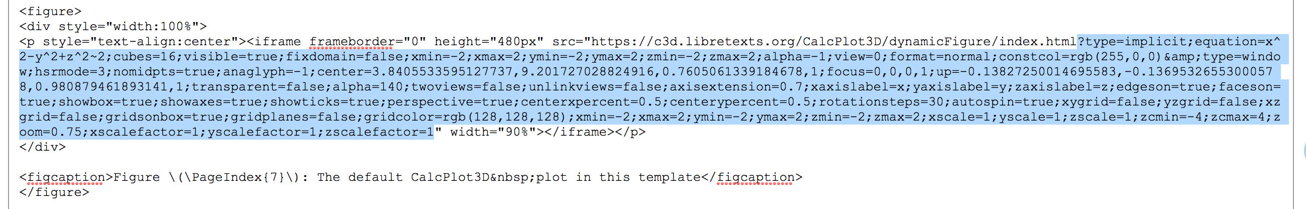
We can also add a CalcPlot3D dynamic figure using the new template, Template:AddFigureCalcPlot3DNew. This template includes the actual HTML code for the CalcPlot3D object so that you can modify the parameters yourself or copy-and-paste the query string from the CalcPlot3D-generated URL into the provided HTML code. Once you have updated the code, you'll also want to remove the instructions given at the top of the figure.
When you insert the template, you will see the following:

To adjust the actual plot shown, you will switch to HTML edit mode using the button in the upper-right corner of the edit window labeled </> HTML. Then you will copy the query string in the URL generated by CalcPlot3D, as described above (everything after the ?) and paste it into the template code, replacing just the query string starting with ? and ending with "zscalefactor=1". See the highlighted portion of the code in Figure \(\PageIndex{10}\) below.
One advantage of this method of inserting your CalcPlot3D dynamic figures is that you can see how they look in the Visual mode as you edit the page.
Rendering the default figure (with the instructions line removed):
Creating your own CalcPlot3D Dynamic Figures using CalcPlot3D (with controls)
Several types of plots in CalcPlot3D can be used to generate dynamic figures that include scrollbars, textboxes or other controls that meaningfully control aspects of the figure.
These are (so far):
- Any plot that uses parameter sliders
- Any space (or plane) curve plot can include sliders and an animate button (as shown in Figure \(\PageIndex{3}\) above).
- Any volume of revolution figure can include a whole set of controls (as shown in Figure \(\PageIndex{2}\) above).
- The trace plane can be shown along with the rotatable 3D plot when contours are shown in the 3D plot, allowing an input point in the trace plane to be moved around while displaying the corresponding output point on the surface. (See Figure \(\PageIndex{12}\) below.)
If you have other situations that you'd like to animate that are not covered here, please send a detailed request of your idea to Paul Seeburger.
Creating the URL Query String in CalcPlot3D for a Dynamic Figure with Controls
To make a CalcPlot3D dynamic figure that includes meaningful controls, it does need to include certain things for this to happen.
If you include parameters and parameter sliders are visible on the control panel when in CalcPlot3D, this plot can be converted into a dynamic figure with controls.
Secondly, as mentioned above, any volume of revolution and any plane curve or space curve can be converted into a dynamic figure with controls.
And finally, if you create a contour plot for a function of two variables and save it to the URL when the main plot window is 3D, but still showing the contours on the surface, then this can be converted into dynamic figure like that shown in Figure \(\PageIndex{12}\) above.
Once you have created your plot in CalcPlot3D, use the process described above in the section titled Creating your own CalcPlot3D Dynamic Figures using CalcPlot3D (without controls). That is, use the Encode View in URL option on the File menu to obtain the query string for the CalcPlot3D plot. Copy the query string to the clipboard, as described above and then follow the instructions below.
Inserting CalcPlot3D Dynamic Figures with Controls in LibreTexts Pages
Creating Sharable CalcPlot3D Dynamic Figures with Controls
First, you will need to either create a copy of a similar CalcPlot3D dynamic figure with controls in your repository folder. If you already have one there, just copy it. If not, copy one from the Learning Objects library, following the steps described in section Creating Sharable CalcPlot3D Interactive Figures in LibreTexts above.
Second, you should check that the figure does indeed use the correct URL to call CalcPlot3D. If it has controls, it should call the following base URL before the query string:
https://c3d.libretexts.org/CalcPlot3D/dynamicFigureWCP/index.html
Note that the only thing that is different here is that the base URL has the characters 'WCP' after 'dynamicFigure' in its path. The WCP represents, "With Control Panel".
Third, you can paste the query string from your CalcPlot3D plot into this new template that you have made.
This means that in order to add a CalcPlot3D dynamic figure with controls, you will either need to copy an existing figure with controls or you will need to modify the HTML base URL by adding these three letters (WCP).
There are a number of special commands you may wish to add to the script in the URL query string to adjust what appears and how it is labeled.
Useful Script Commands for CalcPlot3D Dynamic Figures
For CalcPlot3D dynamic figures with controls there are a few options that you may wish to add to the query string by hand. There are even a few commands listed in the last bullet below that can be used for CalcPlot3D dynamic figures with or without controls.
-
You can add a
nameattribute and/or anoanimateattribute to any sliders. For example, “noanimate=true;name=n_x”. Note that each object, including the sliders, starts with “type=” in the query string. To clarify, these attributes must be set in the definition of the relevant slider object.
See:type=slider;slider=a;value=1;steps=2;pmin=1;pmax=3;repeat=true;bounce=true;waittime=40;careful=true;noanimate=true;name=n_xThe
nameattribute changes the label of the slider to the supplied name, using MathJAX to format the supplied name. This means you can use LaTeX in the name.The
noanimateattribute allows you to hide the Animate button on the slider control, if you wish. -
For figures showing the trace plane (currently those with contour plots), you can add one or more of the following attributes to the window element at the very end of the query string: “hidexysliders=true; hidetracevalue=true;hidetrancepoint=true;”
See:
type=window;hsrmode=3;anaglyph=-1;center=-7.447051206708178,-2.790794355991455,3.71998429905919,1;
focus=0.5,0.5,0.5,1;up=0.39804763218685024,0.14521777837291014,0.9057979241281567,1;transparent=true;alpha=140;twoviews=false;
unlinkviews=false;axisextension=0;xaxislabel=%20;yaxislabel=%20;zaxislabel=%20;edgeson=false;faceson=true;showbox=false;
showaxes=false;showticks=false;perspective=true;centerxpercent=0.5;centerypercent=0.4;rotationsteps=30;autospin=true;
xygrid=false;yzgrid=false;xzgrid=false;gridsonbox=false;gridplanes=true;gridcolor=rgb(128,128,128);
xmin=0;xmax=1;ymin=0;ymax=1;zmin=0;zmax=1;xscale=1;yscale=1;zscale=1;zcmin=-4;zcmax=4;zoom=3.543529;
xscalefactor=1;yscalefactor=1;zscalefactor=0.5;
hidexysliders=true;hidetracevalue=true;hidetracepoint=true;"
width="90%"></iframe></p>
Here the
hidexysliderstag allows you to hide the \(x\)- and \(y\)-sliders that appear below the 2D trace plane by default.The
hidetracevaluetag allows you to hide the trace value normally displayed on the 3D plot when moving a trace point around on the 2D trace plane (and 3D surface).
Thehidetracepointtag allows you to hide the trace point that may otherwise be shown when you click on the 2D trace plane that appears here. -
For figures that include volumes of revolution, you may wish to add the
hideaxisofrevcommand.See:
type=window;hsrmode=0;nomidpts=false;anaglyph=-1;center=5,3,10;focus=0,0,0,1;up=0,2,0;transparent=false; alpha=140;twoviews=false;unlinkviews=false;axisextension=0.7;xaxislabel=x;yaxislabel=y;zaxislabel=z;edgeson=true; faceson=true;showbox=false;showaxes=true;showticks=true;perspective=true;centerxpercent=0.3832428501164356; centerypercent=0.42;rotationsteps=30;autospin=true;xygrid=false;yzgrid=false;xzgrid=false;gridsonbox=true; gridplanes=false;gridcolor=rgb(128,128,128);xmin=-1;xmax=5;ymin=-2;ymax=4;zmin=-4;zmax=4;xscale=1;yscale=1; zscale=2;zcmin=-8;zcmax=8;zoom=0.37;xscalefactor=1;yscalefactor=1;zscalefactor=1; rotatestart=0;rotatedirectionx=1;rotatedirectiony=0;hidexysliders=true;hidetracevalue=true; hidetracepoint=true;hideaxisofrev=false" width="90%"> -
Note the other commands shown here can be used in any CalcPlot3D dynamic figure (with or without controls).
Therotatestartattribute can have values between \(0\) and \(100\) and allows you to set an initial rotation speed. The default speed is 0 which will not cause any initial rotation.The
rotatedirectionxandrotatedirectionyattributes allows you to specify the initial direction of rotation. Typically these values should be between -1 and 1.
Other commands will likely be created as new features are added to CalcPlot3D to accommodate new types of dynamic figures with controls.