2.2: Attributes of Functions

Last updated
Save as PDF

Page ID: 34871

$ \newcommand{\vecs}[1]{\overset { \scriptstyle \rightharpoonup} {\mathbf{#1}} } $ $ \newcommand{\vecd}[1]{\overset{-\!-\!\rightharpoonup}{\vphantom{a}\smash {#1}}} $$\newcommand{\id}{\mathrm{id}}$ $ \newcommand{\Span}{\mathrm{span}}$ $ \newcommand{\kernel}{\mathrm{null}\,}$ $ \newcommand{\range}{\mathrm{range}\,}$ $ \newcommand{\RealPart}{\mathrm{Re}}$ $ \newcommand{\ImaginaryPart}{\mathrm{Im}}$ $ \newcommand{\Argument}{\mathrm{Arg}}$ $ \newcommand{\norm}[1]{\| #1 \|}$ $ \newcommand{\inner}[2]{\langle #1, #2 \rangle}$ $ \newcommand{\Span}{\mathrm{span}}$ $\newcommand{\id}{\mathrm{id}}$ $ \newcommand{\Span}{\mathrm{span}}$ $ \newcommand{\kernel}{\mathrm{null}\,}$ $ \newcommand{\range}{\mathrm{range}\,}$ $ \newcommand{\RealPart}{\mathrm{Re}}$ $ \newcommand{\ImaginaryPart}{\mathrm{Im}}$ $ \newcommand{\Argument}{\mathrm{Arg}}$ $ \newcommand{\norm}[1]{\| #1 \|}$ $ \newcommand{\inner}[2]{\langle #1, #2 \rangle}$ $ \newcommand{\Span}{\mathrm{span}}$$\newcommand{\AA}{\unicode[.8,0]{x212B}}$

Domain and Range

A domain is the largest set of real numbers for which the value of an expression is a real number. Values that must be excluded from a domain include real numbers that cause division by zero and real numbers that result in taking an even root of a negative number. Often the domain is not explicitly stated. However, it is useful to be able to determine what the domain of an expression is.

Domain of a Function

The following steps can be taken to determine what the domain of a function defined by an equation actually is.

$how-to.png$ How to: Find the Domain of a Function Defined by an Equation.

Given a function, $f(x)$, start with the domain as the set of all real numbers.

Radicals with even indexes. If the equation has a radical with an even index (like square root has an index of 2), restrict the domain to only those values of $x$ for which the expression inside the radical (called the radicand) is greater than or equal to zero. To obtain all the intervals that $x$ must be restricted to, solve the $ \underline{\textrm{inequality}} \text{, } \textbf{radicand} \ge 0 $, for each radical with an even index. The result of all these restrictions is the intersection of these intervals.
Denominators. If the equation has a denominator, exclude from the domain any values of $x$ that would make the denominator zero. To obtain all these restrictions, solve the $ \underline{\textrm{equation}} \text{, } \textbf{denominator} \ne 0 $, for each denominator containing variables. Denominators include each expression found below a fraction bar in the equation. Every one of these excluded values must then be removed from the result obtained in step 1.
The result obtained in step 2 is the domain of the equation. Write it in interval form.

Example $\PageIndex{1}$: Find the Domain of a Polynomial Function

Find the domain of the function $f(x)=x^2−1$.

Solution

We start with a domain of all real numbers.
Step 1. The function has no radicals with even indices, so no restrictions to the domain are introduced in this step.
Step 2. The function has no denominators, so no restrictions to the domain are introduced in this step.
Step 3. Thus there are no restrictions on the domain of this function. The domain is the set of real numbers. In interval form, the domain of $f$ is $(−\infty,\infty)$.

Example $\PageIndex{2}$: Find the Domain of a Rational Function

Find the domain of the function $f(x)=\dfrac{x+1}{2−x}$.

Solution

We start with a domain of all real numbers.
Step 1. The function has no radicals with even indices, so no restrictions to the domain are introduced in this step.
Step 2. The function has a denominator, so the domain is restricted such that $2-x \ne 0$. Solving this equation we obtain the restriction to the domiain: $x \ne 2$. In other words the domain is $x<2$ or $x>2$.
Step 3. The domain is all real numbers where $x<2$ or $x>2$. We can use a symbol known as the union, $\cup$, to combine the two sets. In interval notation, the domain is $(−\infty,2)∪(2,\infty)$.

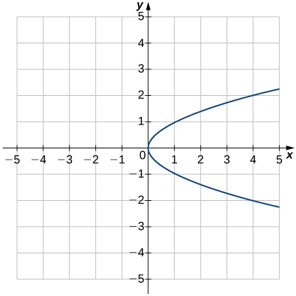
The root functions $f(x)=x^{1/n}$, which can be written as radicals with an index of $n$, have different characteristics depending on whether $n$ is odd or even. For all even integers $n≥2$, the domain of $f(x)=x^{1/n}$ is the interval $[0,∞)$. For all odd integers $n≥1$, the domain of $f(x)=x^{1/n}$ is the set of all real numbers. This is the reason why domains of radical expressions with even indices are restricted and why domains of radical expressions with odd indices have no restrictions.

An image of two graphs. The first graph is labeled “a” and has an x axis that runs from -2 to 9 and a y axis that runs from -4 to 4. The first graph is of two functions. The first function is “f(x) = square root of x”, which is a curved function that begins at the origin and increases. The second function is “f(x) = x to the 4th root”, which is a curved function that begins at the origin and increases, but increases at a slower rate than the first function. The second graph is labeled “b” and has an x axis that runs from -8 to 8 and a y axis that runs from -4 to 4. The second graph is of two functions. The first function is “f(x) = cube root of x”, which is a curved function that increases until the origin, becomes vertical at the origin, and then increases again after the origin. The second function is “f(x) = x to the 5th root”, which is a curved function that increases until the origin, becomes vertical at the origin, and then increases again after the origin, but increases at a slower rate than the first function. 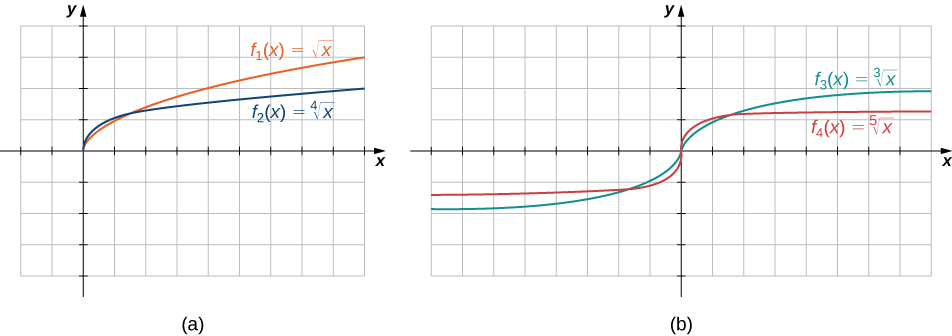— Figure $\PageIndex{7}$: (a) If $n$ is even, the domain of $f(x)=\sqrt[n]{x}$ is $[0,∞)$. (b) If $n$ is odd, the domain of $f(x)=\sqrt[n]{x}$ is $(−∞,∞)$.

Example $\PageIndex{3}$: Find the Domain of a Radical Function

Find the domain of the function $f(x) = \sqrt{7-x}$.

Solution

We start with a domain of all real numbers.
Step 1. The function has a square root, which is a radical with an even index, so the domain is restricted to values of $x$ such that $ 7-x \ge 0.$ Solving this inequality we obtain $-x \ge -7$ or $x \le 7$. At this point the domain has been restricted to all real numbers less than or equal to 7.
Step 2. The function has no denominators, so no further restrictions to the domain are introduced in this step.
Step 3. The domain is the set of real numbers less than or equal to 7. In interval form, the domain of $f$ is $\left(−\infty,7\right]$.

Example $\PageIndex{4}$: Find Domains of Functions

For each of the following functions, determine the domain of the function.

$f(x)=\dfrac{3}{x^2−1} \\ $
$f(x)=\dfrac{2x+5}{3x^2+4} \\ $
$f(x)=\sqrt[3]{2x−1} \\ $

Solution

The function has a denominator and you cannot divide by zero, so the domain is the set of values $x$ such that $x^2−1≠0$. Therefore, the domain is $\{x|x≠±1\}$.
The function has a denominator and you cannot divide by zero, so the domain is the set of values $x$ such that $3x^2+4 \ne 0$. Solving this inequality, we obtain $x^2 \ne -\tfrac{4}{3}.$ Since $x^2≥0$ for all real numbers $x$, the inequality $x^2 \ne -\tfrac{4}{3}$ will be true for any real number chosen for $x$. Therefore, the domain is $(−∞,∞).$
The function does not have an even index (it has a cube root, which has an odd index of $3$, and is defined for all real numbers). The function also does not have a denominator. So the domain is the interval $(−∞, ∞).$

$try-it.png$ Try It $\PageIndex{5}$

Find the domain of the following functions.

a. $f(x)=5−x+x^3$	b. $f(x)=\dfrac{1+4x}{2x−1}$	c. $f(x)=\sqrt{4−3x} $
a. Answer $(−\infty,\infty)$	b. Answer $(−\infty,\dfrac{1}{2})\cup(\dfrac{1}{2},\infty) $	c. Answer $ (-\infty,4/3 ] $

Example $\PageIndex{6}$: More Domains of Functions

For each of the following functions, determine the domain of the function.

a. $f(x)=\sqrt{x-3} + \sqrt{8-x}$

$ \begin{array}{lcll}
\textbf{Solution:} &&&\\
x-3 \ge 0 & {\small{\text{AND}}} & 8-x \ge 0 & \text{Radicands of square roots must be greater than or equal to zero}\\
x \ge 3 && x \le 8 &\text{The domain is the intersection of these intervals}\\
&&& \text{The domain is: } [3, 8] \\
\end{array} $

b. $f(x)=\dfrac{x+1}{x-4}+\dfrac{5x}{x+6}$

$ \begin{array}{lcll}
\textbf{Solution:} &&&\\
x-4 \ne 0 & {\small{\text{AND}}} & x+6 \ne 0 & \text{Denominators cannot be equal to zero}\\
x \ne 4 && x \ne -6 &\text{The domain does not include these values}\\
&&& \text{The domain is: } ( \infty , -6) \cup (-6,4) \cup (4, \infty ) \\
\end{array} $

c. $f(x)=\dfrac{x-9}{\sqrt{x+2}}$

$ \begin{array}{lcll}
\textbf{Solution:} &&&\\
x+2 \ge 0 &&& \text{Radicands of square roots must be greater than or equal to zero}\\
&& \sqrt{x+2} \ne 0 & \text{Denominators cannot be equal to zero}\\
x \ge -2 & {\small{\text{AND}}} & x \ne -2 &\text{Both are restrictions to the domain}\\
&&& \text{The domain is: } (-2, \infty )
\end{array} $

d. $f(x)=\dfrac{1+\tfrac{x+2}{x-3}}{4-\sqrt{x+5}}$

$ \begin{array}{lccll}
\textbf{Solution:} &&&\\
x+5 \ge 0 &&&& \text{Step 1. Radicands of even roots must be } \ge 0\\
x \ge -5 &&&& \text{Resulting Restricted Interval}\\
& x-3 \ne 0 & {\small{\text{AND}}} & 4-\sqrt{x+5} \ne 0 & \text{Step 2. Denominators cannot be equal to zero}\\
& x \ne 3 & {\small{\text{AND}}} & 4 \ne \sqrt{x+5} & \text{Simplify}\\
& & & 16 \ne x+5 & \text{Simplify (square both sides)}\\
& x \ne 3 & {\small{\text{AND}}} & x \ne 11 & \text{Restrictions due to denominators}\\
x \ge -5 \quad {\small{\text{AND}}} & x \ne 3 & {\small{\text{AND}}} & x \ne 11 & \text{All 3 restrictions must be true}\\
&&&& \text{The domain is: } (-5,3) \cup (3,11) \cup (11, \infty )
\end{array} $

$try-it.png$ Try It $\PageIndex{7}$

Find the domain for each of the following functions: $f(x)=(5−2x)/(x^2+2)$ and $g(x)=\sqrt{5x−1}$.

Answer: The domain of $f$ is $(−∞, ∞)$. The domain of $g$ is $ [1/5, \infty )$

Domain and Range of a Graph

$[Graph of a polynomial that shows the x-axis is the domain and the y-axis is the range]$ Another way to identify the domain and range of functions is by using graphs. Because the domain refers to the set of possible input values, the domain of a graph consists of all the input values shown on the $x$-axis. The range is the set of possible output values, which are shown on the $y$-axis. Keep in mind that if the graph continues beyond the portion of the graph we can see, the domain and range may be greater than the visible values. This is illustrated in the figure at the right.

We can observe that the graph extends horizontally from −5 to the right without bound, so the domain is $\left[−5,∞\right)$. The vertical extent of the graph is all range values 5 and below, so the range is $\left(−∞,5\right]$. Note that the domain and range are always written from smaller to larger values, or from left to right for domain, and from the bottom of the graph to the top of the graph for range.

Example $\PageIndex{8}$: Find Domain and Range from a Graph

Find the domain and range of the function $f$ whose graph is shown below

Solution

We can observe that the horizontal extent of the graph is –3 to 1, so the domain of $f$ is $\left(−3,1\right]$. The vertical extent of the graph is between 0 and –4, so the range is $\left[−4,0\right]$. (Because (0,0) is a point on the graph, $y=0$ needs to be included in the range). This is illustrated below.

[Graph of the previous function shows the domain and range.]

$try-it.png$ Try It $\PageIndex{8}$

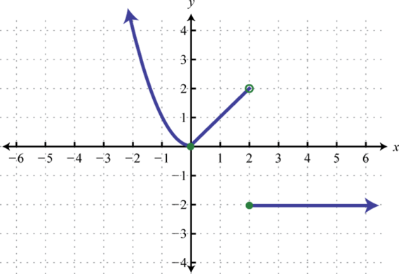
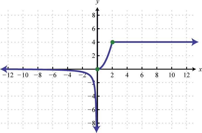
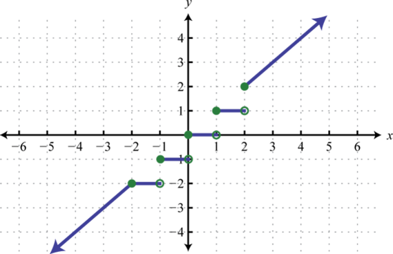
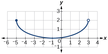
Find the domain and range of the functions illustrated in the graphs below.

a)	b)	c)
$Graph of a function from $\left(2, 8\right]$.$	$Graph of a function from (-infinity, 2].$
d) Asymptotes at x=0 and y=0	e)	f) Open circle at (0,2)

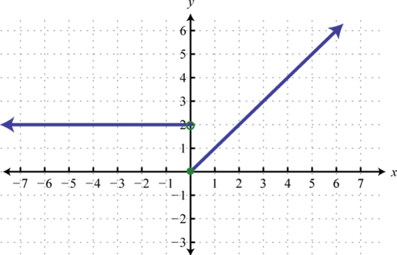g) Open circles at (2,2) and (2,-2)	h) Asymptote at $x=0,$ filled circle at (0,0)	i) Each horizontal segment ends in an open circle

a. Answer Domain: $ (2, 8] $ Range: $ [6, 8) $	b. Answer Domain: $ (-\infty, 1] $ Range: $ [0,\infty) $	c. Answer Domain: $ (−\infty,\infty) $ Range: $ (−\infty,\infty) $
d. Answer Domain: $ (−\infty,0) \cup (0,\infty) $ Range: $ (−\infty,0) \cup (0,\infty) $	e. Answer Domain: $(−\infty,\infty)$ Range: $ [0,\infty) $	f. Answer Domain: $(−\infty,\infty)$ Range: $ [0,\infty) $
g. Answer Domain: $(−\infty,2) \cup (2,\infty) $ Range: $ [-2,-2] \cup [0,\infty) $	h. Answer Domain: $ (−\infty,\infty) $ Range: $ (−\infty, \infty) $	i. Answer Domain: $ (−\infty,\infty) $ Range: $ (-\infty, -2] \cup [-1,-1] \cup [0,0] \cup [1,1] \cup [2,\infty) $

Construct a Graph from a Table of Values

One way to describe relations is with equations. Visualizations of equations can be done using graphs.

The Fundamental Graphing Principle

The graph of an equation is the set of points which satisfy the equation. That is, a point $ (x,y)$ is on the graph of an equation if and only if $x$ and $y$ satisfy the equation.

Here, `$x$ and $y$ satisfy the equation' means `$x$ and $y$ make the equation true'. If the equation to be graphed contains both $x$ and $y$, then the equation defines the relationship between the two variables. The points $ (x,y)$ that we graph are the pairs of $x$ and $y$ which make the equation true.

Example $\PageIndex{9}$: Determine if a point is on a graph

Determine whether or not $(2,-1)$ is on the graph of $x^2 + y^3 = 1$

$ {\bf Solution.} $ We substitute $x=2$ and $y=-1$ into the equation to see if the equation is satisfied.

\[ \begin{array}{rclr} (2)^2+(-1)^3 & \stackrel{?}{=} & 1 & \\3 & \neq & 1 & \nonumber \end{array} \]

Hence, $(2,-1)$ is $ \textbf{not}$ on the graph of $x^2 + y^3 = 1$ because substituting $x=2$ and $y=-1$ into the equation results in a statement that is not true.

Example $\PageIndex{10}$: Construct a graph using a table of values

Graph $x^2 + y^3 = 1$

$ {\bf Solution.} $ Step 1. To efficiently generate points on the graph of this equation, we first solve for $y$

\[ \begin{array}{rclr} x^2 + y^3 & = & 1 & \\ y^3 & = & 1 - x^2 & \\ \sqrt[3]{y^3} & = & \sqrt[3]{1 - x^2} & \\ y & = & \sqrt[3]{1 - x^2} \nonumber \\ \end{array} \]

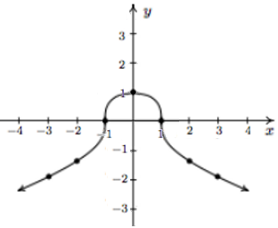
Step 2. Choose values for $x$ and calculate corresponding values for $y$. Plot the resulting point $(x,y)$. For example, substituting $x=-3$ into the equation yields $y = \sqrt[3]{1 - x^2} = \sqrt[3]{1 - (-3)^2} = \sqrt[3]{-8} = - 2,$ so the point $(-3, -2)$ is on the graph. Continuing in this manner, we generate a table of points which are on the graph of the equation. These points are then plotted in the plane as shown below.

\[\begin{array}{|r||c|c|} \hline x & y & (x,y) \\ \hline -3 & -2 & (-3, -2) \\ \hline -2 & -\sqrt[3]{3}& (-2,-\sqrt[3]{3}) \\ \hline -1 & 0 & ( -1, 0) \\ \hline 0 & 1& ( 0 , 1) \\ \hline 1 & 0 & ( 1, 0) \\ \hline 2 & -\sqrt[3]{3}& (2,-\sqrt[3]{3}) \\ \hline 3 & -2 & (3, -2) \\ \hline \end{array} \nonumber\]

Table of values

$2.1 graph of cubeRoot(1-xSquared) dots.png$

Plotted Points

$2.1 graph of cubeRoot(1-xSquared) curve.png$

Connected 'Dots'

These points constitute only a small sampling of the points on the graph of this equation. To get a better idea of the shape of the graph, we could plot more points until we feel comfortable `connecting the dots'. Doing so would result in a curve similar to the one pictured above on the far right.

It should be mentioned here that it is entirely possible to choose a value for $x$ which does not correspond to a point on the graph. For example, if we were plotting points for the equation $y = \sqrt{1-(x-2)^2}$ and substituted $x=0$ into the equation, we would obtain $y = \sqrt{1 - (0-2)^2} = \sqrt{1 - 4} = \sqrt{-3},$ which is not a real number. This means there are no points on the graph with an $x$-coordinate of $0.$ When this happens, we move on and try another point. This is a drawback of the `plug-and-plot' approach to graphing equations. Soon we will develop techniques which allow us to graph entire families of equations quickly (and without the use of a calculator!)

Zeros and Intercepts

Of all of the points on the graph of an equation, the places where the graph touches or crosses the axes hold special significance. These are called the intercepts of the graph. Intercepts come in two distinct varieties: $x$-intercepts and $y$-intercepts. They are defined below.

Definition: Zeros and Intercepts

Zeros are all the real and imaginary values of $x$ that are solutions to the equation $ y=0 $. Zeros are typically listed in set notation.

$x$-intercepts are the points on the $x$ axis where a graph touches or crosses the $x$ axis. They are all the real number values of $x$ for which $ y=0 $. The $y$ coordinate corresponding to an $x$-intercept is always zero. $x$-intercepts are written as coordinate points in the form $ (a,0) $.

$y$-intercepts are the points on the $y$ axis where a graph touches or crosses the $y$ axis. They are all the real number values of $y$ for which $ x=0 $. The $x$ coordinate corresponding to an $y$-intercept is always zero. Functions can have at most one $y$-intercept. $y$-intercepts are written as coordinate points in the form $ (0,b) $.

In our previous example the graph had two $x$-intercepts, $(-1,0)$ and $(1,0)$, and one $y$-intercept, $(0,1)$. The graph of an equation can have any number of intercepts, including none at all!

Zeros and Intercepts from a Graph

$how-to.png$ How to: Find Zeros and Intercepts from a graph.

$x$-intercepts are the points $ (a,0) $ where the graph touches or crosses the $x$-axis
$y$-intercepts are the points $(0,b)$ where the graph touches or crosses the $y$-axis
Only real number zeros are visible on a graph. Imaginary zeros are not visible on a graph.

Example $\PageIndex{11}$: Zeros and Intercepts on a Graph

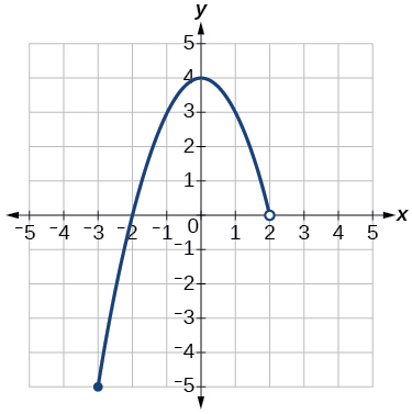
For each function graphed below, find the zeros, $x$-intercepts, and $y$-intercept.

a.
$Graph of a function [-5,3)$

b.
$Graph of a function from [-3, 2).$

Solution. Graphs only show real number zeros. A graph cannot supply any information about the existence of imaginary zeros.

a. visible zeros: { -1 }, $x$-intercepts: (-1, 0), $y$-intercept: (0, .1) approximately
b. visible zeros: { -2 }, $x$-intercepts: (-2, 0), $y$-intercept: (0, 4)

Zeros and Intercepts from an Equation

Since $x$-intercepts lie on the $x$-axis, we can find them by setting $y = 0$ in the equation. Similarly, since $y$-intercepts lie on the $y$-axis, we can find them by setting $x = 0$ in the equation. Keep in mind, intercepts are points and therefore must be written as ordered pairs. To summarize,

$how-to.png$ How to: Find Zeros and Intercepts given an Equation.

Given an equation involving $x$ and $y$

Zeros are written as the set $\{z_1, z_2,...\}$ of all the solutions obtained for $x$ when $y=0$ is substituted into the equation.
$x$-intercepts have the form $(x,0)$. Set $y=0$ in the equation and solve for $x$. The $x$-intercepts are the real number solutions found. Imaginary number solutions and solutions that are not in the domain are NOT included.
$y$-intercepts have the form $(0,y)$. Set $x=0$ in the equation and solve for $y$. The $y$-intercepts are the real number solutions found.

Example $\PageIndex{12}$: Find Zeros and Intercepts given an Equation

Find the $x$- and $y$-intercepts (if any) of the graph of $(x-2)^2 + y^2 = 1$.

Solution

To look for $x$-intercepts, we set $y=0$ and solve to find the zeros:

\[ \begin{array}{rclr} (x-2)^2 + y^2 & = & 1 & \\ (x-2)^2 + 0^2 & = & 1 & \\ (x-2)^2 & = & 1 & \\ \sqrt{(x-2)^2} & = & \sqrt{1} & \mbox{extract square roots}\\ x - 2 & = & \pm 1 & \\ x & = & 2 \pm 1 & \\ x & = & 3, 1 \nonumber \end{array} \]

We get two answers for $x$ so the zeros are $\{1,\;3\}$, which correspond to two $x$-intercepts: $(1,0)$ and $(3,0)$.

Turning our attention to $y$-intercepts, we set $x=0$ and solve:

\[ \begin{array}{rclr} (x-2)^2 + y^2 & = & 1 & \\ (0-2)^2 + y^2 & = & 1 & \\ 4 + y^2 & = & 1 & \\ y^2 & = & -3 \nonumber \end{array} \]

Since there is no real number which squares to a negative number, we are forced to conclude that the graph has no $y$-intercepts.

Zeros and Intercepts from a Function

$how-to.png$ How to: Find Zeros and Intercepts given a Function.

Given a function $f(x)$

Zeros are written as the set $\{z_1, z_2,...\}$ of all the solutions obtained for the equation $f(x) = 0$. Results that are not in the domain are not considered to be solutions.
$x$-intercepts have the form $(x,0)$. $x$-intercepts include only the subset of zeros that are real numbers. Imaginary zeros are not included.
The $y$-intercept is the point $(0,f(0))$. A function has at most one $y$-intercept.

Example $\PageIndex{13}$: Find Zeros and Intercepts given a Function

For each function below, (a) Find all the zeros and $x$ intercepts of $f$, and (b) Find the $y$-intercept (if any).

$f(x)=−4x+2.$
$f(x)=\sqrt{x+3}+1$.

Solution

1. (a) To find the zeros, solve $f(x)=0$: $−4x+2=0 \longrightarrow 2 = 4x \longrightarrow x=1/2$.
The zeros of $f$ are $\{1/2\}$. The $x$-intercept is $(1/2,0).$

(b) The $y$-intercept is given by $(0,f(0)).$ $f(0) = -4(0)+2 = 2.$ Therefore the $y$-intercept is $(0,2).$

2. (a) To find the zeros, solve $\sqrt{x+3}+1=0$. This equation implies $\sqrt{x+3}=−1$.
Since $\sqrt{x+3}≥0$ for all $x$, this equation has no solutions, and therefore $f$ has no zeros and no $x$-intercepts.

(b) The $y$-intercept is given by $(0,f(0))=(0,\sqrt{3}+1)$.

Example $\PageIndex{14}$

For each function below, find the zeros, $x$-intercepts, and $y$-intercept.

a. $f(x)=1-x+\sqrt{2x+6}$

$ \begin{array}{llll}
\textbf{Solution:} & \text{Solve: } 1-x+\sqrt{2x+6}=0 & &\\
\text{Zeros:} &
\rightarrow \sqrt{2x+6}=x-1
\:\: \rightarrow 2x+6=x^2-2x+1
& \text{Zeros: } \{ 5 \} \\
& \rightarrow x^2-4x-5=0
\:\: \rightarrow (x-5)(x+1)=0
\:\: \rightarrow x=5, x=-1
& x\text{-intercepts: (5,0)} \\
& x=-1 \text{ must be rejected because } \sqrt{2(-1)+6 } \ne -1-1 \\
y\text{-intercept:}& f(0)=1-0+\sqrt{0+6}+1 &y\text{-intercept: } (0, 1+\sqrt{6} ) \\
\end{array} $

In this example notice that because the process of solving involved squaring, the solutions ($x=-1$ and $x=5$) had to be checked.

b. $g(x)=\sqrt{8x−1}$

$ \begin{array}{llll}
\textbf{Solution:} &&&\\
\text{Zeros:} & \text{Solve: } \sqrt{8x−1}=0 & \text{Zeros:}& {\large\{} \tfrac{1}{8} {\large\}} \\
& 8x-1=0 &x\text{-intercepts:} & {\large(} \tfrac{1}{8}, 0 {\large)} \\
& 8x=1 \:\: \rightarrow \:\: x=1/8\\
y\text{-intercept:}& f(0)=\sqrt{0-1} = i &y\text{-intercept:} &\text{none}\\
\end{array} $

c. $g(x)=\dfrac{3}{x}$

$ \begin{array}{llll}
\textbf{Solution:} &&&\\
\text{Zeros:} & \text{Solve: } \dfrac{3}{x}=0 & \text{Zeros:}& \text{None} \\
& (x) \cdot \dfrac{3}{x}=0 \cdot (x) &x\text{-intercepts:} & \text{None} \\
& 3=0 \:\: \rightarrow \:\: \text{No solution}\\
y\text{-intercept:}& f(0)=\dfrac{3}{0}=\text{Undefined} &y\text{-intercept:} & \text{None} \\
\end{array} $

d. $h(x)=\dfrac{x^2+9}{x^2+4} $

$ \begin{array}{llll}
\textbf{Solution:} &&&\\
\text{Zeros:} & \text{Solve: } \dfrac{x^2+9}{x^2+4}=0 & \text{Zeros:}& \{ 3i, -3i \} \\
& (x^2+4) \cdot \dfrac{x^2+9}{x^2+4}=0 \cdot (x^2+4) &x\text{-intercepts:} & \text{None} \\
& x^2+9=0 \:\: \rightarrow \:\: x^2=-9 \:\: \rightarrow \:\: x=\pm \sqrt{-9}\\
y\text{-intercept:}& f(0)=\dfrac{0+9}{0+4}=\dfrac{9}{4} &y\text{-intercept:} & {\LARGE(}0, \dfrac{9}{4} {\LARGE)} \\
\end{array} $

$try-it.png$ Try It $\PageIndex{15}$: Find zeros and Intercepts given a function

Find the zeros of $f(x)=x^3−5x^2+6x.$

Answer: $x=0,2,3$

Symmetry

The graphs of certain functions have symmetry properties that help us understand the function and the shape of its graph.

Definition: Symmetry

Symmetry with respect to the $x$-axis. For every point $(x,y)$ on the graph, point $(x,-y)$ is also on the graph.
Symmetry with respect to the $y$-axis. For every point $(x,y)$ on the graph, point $(-x,y)$ is also on the graph.
Symmetry with respect to the origin. For every point $(x,y)$ on the graph, point $(-x,-y)$ is also on the graph.

Symmetry from a Graph

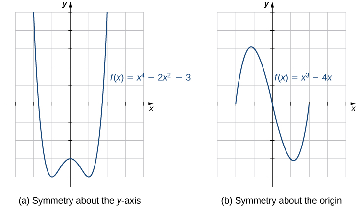
Consider the function $f(x)=x^4−2x^2−3$ shown in the figure $\PageIndex{16a}$ below. If we take the part of the curve that lies to the right of the $y$-axis and flip it over the $y$-axis, it lies exactly on top of the curve to the left of the $y$-axis. In this case, we say the function has symmetry about the $y$-axis.

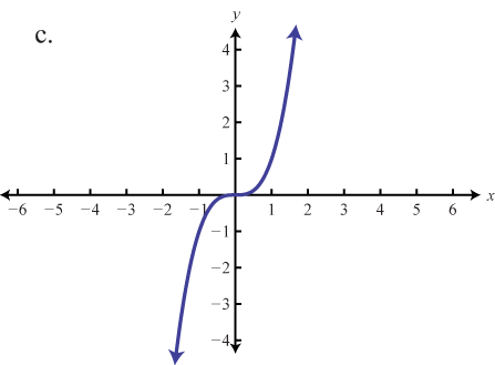
On the other hand, consider the function $f(x)=x^3−4x$ shown in Figure $\PageIndex{16b}$. If we take the graph and rotate it $180°$ about the origin, the new graph will look exactly the same. In this case, we say the function has symmetry about the origin.

If we take the part of the curve in in Figure $\PageIndex{16c}$ that is above the $x$-axis and flip it over the $x$-axis, it will lie exactly on top of the curve that is below the $x$-axis. In this case, the graph has symmetry about the $x$-axis. Unlike the other two examples, the graph is not that of a function, since it fails the vertical line test. Graphs with $x$-axis symmetry are never functions.

Figure $\PageIndex{16}$: Illustration of various types of symmetry

$An image of two graphs. The first graph is labeled “(a), symmetry about the y-axis” and is of the curved function “f(x) = (x to the 4th) - 2(x squared) - 3”. The x axis runs from -3 to 4 and the y axis runs from -4 to 5. This function decreases until it hits the point (-1, -4), which is minimum of the function. Then the graph increases to the point (0,3), which is a local maximum. Then the the graph decreases until it hits the point (1, -4), before it increases again. The second graph is labeled “(b), symmetry about the origin” and is of the curved function “f(x) = x cubed - 4x”. The x axis runs from -3 to 4 and the y axis runs from -4 to 5. The graph of the function starts at the x intercept at (-2, 0) and increases until the approximate point of (-1.2, 3.1). The function then decreases, passing through the origin, until it hits the approximate point of (1.2, -3.1). The function then begins to increase again and has another x intercept at (2, 0).$

$An image of a graph. The x axis runs from -5 to 5 and the y axis runs from -5 to 5. The graph is of a relation that is a sideways parabola, opening up to the right. The x intercept and y intercept are both at the origin and the relation has no points to the left of the y axis. The relation includes the points (1, -1) and (1, 1)$

Example $\PageIndex{16}$

Determine the type(s) of symmetry for each graph.

$symmetryExampleC.gif$

$symmetryExampleB.gif$

Solution: 1. Origin symmetry, 2. $x$-axis symmetry, $y$-axis symmetry, and origin symmetry

Symmetry of an Equation

We have defined symmetry from a graphical perspective, but the ideas can also be applied to equations. For example, the graph we obtained for $x^2 + y^3 = 1$ in Example $\PageIndex{10}$ appears to be symmetric about the $y$-axis. To actually show this algebraically, we assume $(x,y)$ is a generic point on the graph of the equation. That is, we assume $x^2 + y^3 = 1$ is true. The point symmetric to $(x,y)$ about the $y$-axis is $(-x,y)$ To show that the graph is symmetric about the $y$-axis, we need to show that $(-x,y)$ satisfies the equation $x^2 + y^3 = 1$ too. Substituting $(-x,y)$ into the equation gives

$ \begin{array}{rclr} (-x)^2+(y)^3 & \stackrel{?}{=} & 1 & \\ x^2 + y^3 & \stackrel{\checkmark}{=} & 1 \end{array} $

Since we are assuming the original equation $x^2 + y^3 = 1$ is true, we have shown that $(-x, y)$ satisfies the equation (since it leads to a true result) and hence is on the graph.

In this way, we can check whether the graph of a given equation possesses $x$-axis, $y$-axis, or origin symmetry.

$how-to.png$ How to: Test the Symmetry of an Equation

Given an equation in $x$ and $y$, perform each of the following substitutions to assess the symmetry of the graph of the given equation.

$y$-axis symmetry exists if substituting $-x$ for $x$ results in an equivalent equation.
$x$-axis symmetry exists if substituting $-y$ for $y$ results in an equivalent equation.
origin symmetry exists if substituting both $-x$ for $x$ and $−y$ for $y$ results in an equivalent equation.

It is possible for the graph of an equation to have all three types of symmetry.

Example $\PageIndex{17}$: Find Symmetry given an Equation

Determine the symmetry of the graphs for each equation.

$ 9x^2=4y^2+18xy+27 $
$ | y^3+2y | = 4 | x^2-5 | $

Solution

a. $ 9x^2=4y^2+18xy+27 \qquad$ Answer: The graph of the equation has origin symmetry:

Test for $y$-axis symmetry. $ 9(-x)^2=4y^2+18(-x)y+27 \:\: \rightarrow \:\: 9x^2=4y^2-18xy+27 $, which is not an equivalent equation, so the graph of the equation does not have $y$-axis symmetry.
Test for $x$-axis symmetry. $ 9x^2=4(-y)^2+18x(-y)+27 \:\: \rightarrow \:\: 9x^2=4y^2-18xy+27 $, which is not an equivalent equation, so the graph of the equation does not have $x$-axis symmetry.
Test for origin symmetry. $ 9(-x)^2=4(-y)^2+18(-x)(-y)+27 \:\: \rightarrow \:\: 9x^2=4y^2+18xy+27 $, which is an equivalent equation, so the graph of the equation has origin symmetry.

b. $ | y^3+2y | = 4 | x^2-5 | \qquad$ Answer: The graph of the equation has $y$-axis, $x$-axis and origin symmetry:

Test for $y$-axis symmetry. $ | y^3+2y | = 4 | (-x)^2-5 | \:\: \rightarrow \:\: | y^3+2y | = 4 | x^2-5 | $, which is an equivalent equation, so the graph of the equation has $y$-axis symmetry.
Test for $x$-axis symmetry. $ | (-y)^3+2(-y) | = 4 | x^2-5 | \:\: \rightarrow \:\: | -y^3-2y | = 4 | x^2-5 | \:\: \rightarrow \:\: | -(y^3+2y) | = 4 | x^2-5 |$ $ \:\: \rightarrow \:\: | y^3+2y | = 4 | x^2-5 | $, which is an equivalent equation, so the graph of the equation has $x$-axis symmetry.
Test for origin symmetry produces an equivalent equation, so the graph of the equation has origin symmetry: $ | (-y)^3+2(-y) | = 4 | (-x)^2-5 | \:\: \rightarrow \:\: | -y^3-2y | = 4 | x^2-5 | \:\: \rightarrow \:\: | -(y^3+2y) | = 4 | x^2-5 | \:\: \rightarrow \:\: | y^3+2y | = 4 | x^2-5 | $

Note that in a situation where an equation has been shown to have two of the three types of symmetry, then it must have all three types of symmetry.

$try-it.png$ Try It $\PageIndex{17}$: Test an equation for symmetry

Test the equation $(x-2)^2 + y^2 = 1$ for symmetry.

Answer: The graph is symmetric about the $x$-axis. This means we can cut our `plug and plot' time to graph the equation in half: whatever happens below the $x$-axis is reflected above the $x$-axis, and vice-versa.

Symmetry of a Function; Odd and Even Functions

Sometimes we are given a function in the form $ y = f(x) $. Looking at Figure $\PageIndex{16a}$, we see that since $f$ is symmetric about the $y$-axis, if the point $(x,y)$ is on the graph, the point $(−x,y)$ is also on the graph. In other words, $f(x) = y$ and $f(-x) = y$ so $f(−x)=f(x)$. If a function $f$ has this property, we say $f$ is an even function. All even functions have $y$-axis symmetry. The function $f(x)=x^2$ is even because $f(−x)=(−x)^2=x^2=f(x).$

In contrast, looking at Figure $\PageIndex{16b}$, if a function $f$ is symmetric about the origin, then whenever the point $(x,y)$ is on the graph, the point $(−x,−y)$ is also on the graph. In other words, $f(x) = y$ and $f(-x) = -y$. Since $f(x) = y$ can be rewritten $-f(x)=-y$, we can conclude (f(−x)=−f(x)\). If $f$ has this property, we say $f$ is an odd function. All odd functions have symmetry about the origin. The function $f(x)=x^3$ is odd because $f(−x)=(−x)^3=−x^3=−f(x). $

Definition: Even and Odd Functions

If $f(x)=f(−x)$ for all $x$ in the domain of $f$, then $f$ is an even function. An even function is symmetric about the $y$-axis.
If $f(−x)=−f(x)$ for all $x$ in the domain of $f$, then $f$ is an odd function. An odd function is symmetric about the origin.

Looking at these definitions, it is clear that being able to simplify various functions that have an argument of $-x$ is important. The practice exercise below illustrates some of these needed skills.

$try-it.png$ Try It $\PageIndex{18}$

Simplify the following expressions if possible. Write the final result as an expression that does not have any parentheses.

a. $(-x) $

b. $ (-x)^2$

c. $ (-x)^3$

d. $ (-x)^4$

e. $(-x)^5 $

f. $ |(-x)|$

g. $ \sqrt{(-x)}$

h. $ \sqrt[3]{(-x)}$

i. $ \sqrt[4]{(-x)}$

j. $ \sqrt[5]{(-x)}$

Answer: a. $-x \quad $ b. $x^2 \quad $ c. $-x^3\quad $ d. $x^4\quad $ e. $-x^5\quad $ f. $|x|\quad $ g. $ \sqrt{-x}\quad $ h. $-\sqrt[3]{x}\quad $ i. $\sqrt[4]{-x}\quad $ j. $-\sqrt[5]{x} $

$how-to.png$ How to: Determine if a Function is Even or Odd, and what Kind of Symmetry it Has.

Evaluate $f(−x) $ and simplify it.
Compare the result with $f(x)$ and $−f(x)$
1. If $f(x)=f(−x)$ then $f$ is an even function and has $y$-axis symmetry.
2. If $f(−x)=−f(x)$ then $f$ is an odd function and has origin symmetry.

Any function (except the function $f(x)=0$ ) cannot be both even and odd.
Any function (except the function $f(x)=0$ ) can never have $x$-axis symmetry.

Example $\PageIndex{19}$: Even and Odd Functions

Determine whether each of the following functions is even, odd, or neither, and state the type of symmetry it has.

$f(x)=−5x^4+7x^2−2$
$f(x)=2x^5−4x+5$
$f(x)=\dfrac{3x}{x^2+1}$

Solution

To determine whether a function is even or odd, we evaluate $f(−x)$ and compare it to $f(x)$ and $−f(x)$.

$f(−x)=−5(−x)^4+7(−x)^2−2=−5x^4+7x^2−2=f(x)$. Therefore, $f$ is even, and symmetric about the $y$-axis.
$f(−x)=2(−x)^5−4(−x)+5=−2x^5+4x+5$. Now, $f(−x)≠f(x)$. Furthermore, noting that $−f(x)=−2x^5+4x−5$, we see that $f(−x)≠−f(x)$. Therefore, $f$ is neither even nor odd, and so has neither $y$-axis nor origin symmetry.
$f(−x)=\dfrac{3(−x)}{(−x)2+1}$ $=\dfrac{−3x}{x^2+1}=$ $−\dfrac{3x}{x^2+1}=−f(x)$. Therefore, $f$ is odd, and is symmetric about the origin.

$try-it.png$ Try It $\PageIndex{19}$

Determine whether $f(x)=4x^3−5x$ is even, odd, or neither.

Answer
$f(x)$ is odd.

More Attributes Observable in a Graph

Increasing, Decreasing, or Constant

As part of exploring how functions change, we can identify intervals over which the function is changing in specific ways. We say that a function is increasing on an interval if the function values increase as the input values increase within that interval. Similarly, a function is decreasing on an interval if the function values decrease as the input values increase over that interval.

Definition: Increasing and Decreasing

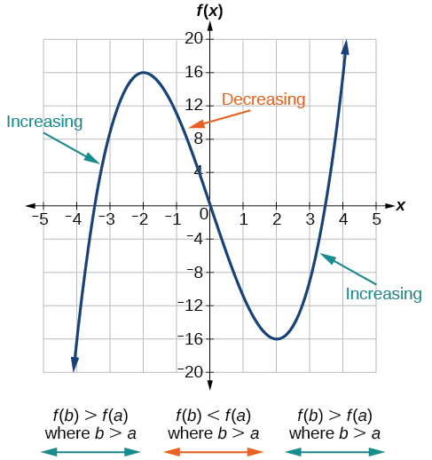
A function $f$ is an increasing function on an open interval $ (a,b) $ where $b>a$, if $f(b)>f(a)$ for every $a$ and $b$ in the interval.
A function $f$ is a decreasing function on an open interval $ (a,b) $ where $b>a$, if $f(b)<f(a)$ for every $a$ and $b$ in the interval.
A function $f$ is a constant function on an open interval $ (a,b) $ where $b>a$, if $f(b)= f(a)$ for every $a$ and $b$ in the interval.

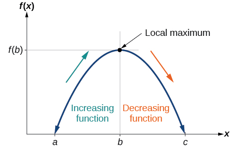
Figure $\PageIndex{20}$ shows examples of increasing and decreasing intervals on a function.

Graph of a polynomial that shows the increasing and decreasing intervals and local maximum and minimum. — Figure $\PageIndex{20}$: The function $f(x)=x^3−12x$ is increasing on $(−\infty, −2) $ and $ (2,\infty)$ and is decreasing on $(−2, 2)$.

Example $\PageIndex{20}$: Find Increasing and Decreasing Intervals on a Graph.

Given the function $p(t)$ in the figure below, identify the intervals on which the function appears to be increasing.

Solution

The function is not constant on any interval. The function is increasing where it slants upward as we move to the right and decreasing where it slants downward as we move to the right. The function appears to be increasing from $t=1$ to $t=3$ and from $t=4$ on. In interval notation, we would say the function appears to be increasing on the interval $(1,3)$ and the interval $(4,\infty)$.

Analysis. Notice in this example that we used open intervals (intervals that do not include the endpoints), because the function is neither increasing nor decreasing at $t=1$, $t=3$, and $t=4$. These points are the local extrema (two minima and a maximum) instead.

Local Maxima and Minima

While some functions are increasing (or decreasing) over their entire domain, many others are not. A value of the input where a function changes from increasing to decreasing (as we go from left to right, that is, as the input variable increases) is called a local maximum. If a function has more than one, we say it has local maxima. Similarly, a value of the input where a function changes from decreasing to increasing as the input variable increases is called a local minimum. The plural form is “local minima.” Together, local maxima and minima are called local extrema, or local extreme values, of the function. (The singular form is “extremum.”) The term "relative extrema", rather than "local extrema" is often used.

Clearly, a function is neither increasing nor decreasing on an interval where it is constant. A function is also neither increasing nor decreasing at extrema. Note that we have to speak of local extrema, because any given local extremum as defined here is not necessarily the highest maximum or lowest minimum in the function’s entire domain.

For the function whose graph is shown in Figure $\PageIndex{21}$, the local maximum is 16, and it occurs at $x=−2$. The local minimum is −16 and it occurs at $x=2$.

Graph of a polynomial that shows the increasing and decreasing intervals and local maximum.] Definition of a local maximum — Figure $\PageIndex{21}$: Graph of a polynomial that shows the increasing and decreasing intervals and local minimum/maximum

To locate the local maxima and minima from a graph, we need to observe the graph to determine where the graph attains its highest and lowest points, respectively, within an open interval. Like the summit of a roller coaster, the graph of a function is higher at a local maximum than at nearby points on both sides. The graph will also be lower at a local minimum than at neighboring points. Figure $\PageIndex{22}$ illustrates these ideas for a local maximum.

Graph of a polynomial that shows the increasing and decreasing intervals and local maximum. — Figure $\PageIndex{22}$: Definition of a local maximum

These observations lead us to a formal definition of local extrema.

Definition: Local Minima and Local Maxima

A function $f$ has a local maximum at a point $b$ in an open interval $(a,c)$ if $f(b)$ is greater than or equal to $f(x)$ for every point $x$ ($x$ does not equal $b$) in the interval. The maximum is at $x=b$; the maximum is $y=f(b)$.

A function $f$ has a local minimum at a point $b$ in an open interval $(a,c)$ if $f(b)$ is less than or equal to $f(x)$ for every $x$ ($x$ does not equal $b$) in the interval. The minimum is at $x=b$; the minimum is $y=f(b)$.

Local extrema are also called relative extrema.

Example $\PageIndex{23}$: Find Local Maxima and Minima from a Graph

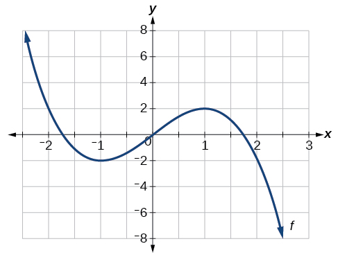
For the function $f$ whose graph is shown in the figure below, find all local maxima and minima.

Solution

Observe the graph of $f$. The graph attains a local maximum at $x=1$ because it is the highest point in an open interval around $x=1$. The local maximum is the $y$-coordinate at $x=1$, which is $2$.

The graph attains a local minimum at $x=−1$ because it is the lowest point in an open interval around $x=−1$. The local minimum is the $y$-coordinate at $x=−1$, which is $−2$.

Absolute Maxima and Minima

There is a difference between locating the highest and lowest points on a graph in a region around an open interval (locally) and locating the highest and lowest points on the graph for the entire domain. The $y$-coordinates (output) at the highest and lowest points are called the absolute maximum and absolute minimum, respectively. To locate absolute maxima and minima from a graph, we need to observe the graph to determine where the graph attains it highest and lowest points on the domain of the function.

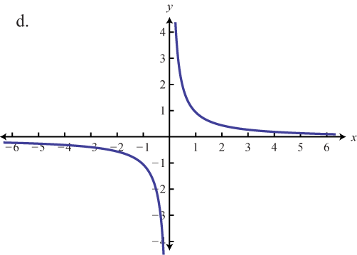
Graph of a segment of a parabola with an absolute minimum at (0, -2) and absolute maximum at (2, 2).

Not every function has an absolute maximum or minimum value. The function $f(x)=x^3$ is one such function.

Definition: Absolute Minima and Absolute Maxima

The absolute maximum of $f$ at $x=c$ is $f(c)$ where $f(c)≥f(x)$ for all $x$ in the domain of $f$.
The absolute minimum of $f$ at $x=d$ is $f(d)$ where $f(d)≤f(x)$ for all $x$ in the domain of $f$.

Absolute extrema are also called global extrema.

Example $\PageIndex{24}$: Find Absolute Maxima and Minima from a Graph

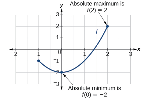
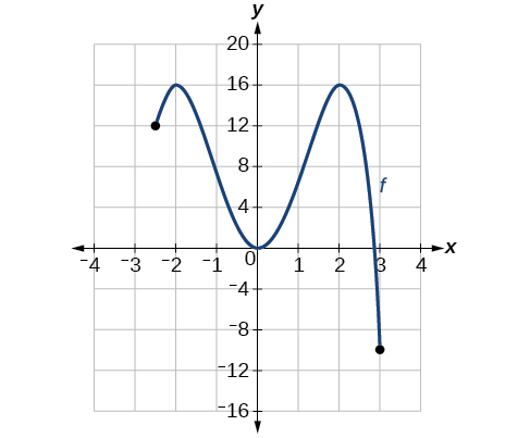
For the function $f$ shown in Figure $\PageIndex{24}$, find all absolute maxima and minima.

Solution

Observe the graph of $f$. The graph attains an absolute maximum in two locations, $x=−2$ and $x=2$, because at these locations, the graph attains its highest point on the domain of the function. The absolute maximum is the $y$-coordinate at $x=−2$ and $x=2$, which is $16$.

The graph attains an absolute minimum at $x=3$, because it is the lowest point on the domain of the function’s graph. The absolute minimum is the $y$-coordinate at $x=3$, which is $−10$.

We can see the difference between local and global extrema in Figure $\PageIndex{25}$ below. In this example, $y=5$ is both a local maximum and a global maximum. The graph does NOT have a global minimum because $y = -\infty $ is not a finite real number value and it ( $ -\infty $ ) is not in the range of $f$ since the range is $ (-\infty, 5] $ which does not include $ -\infty$!

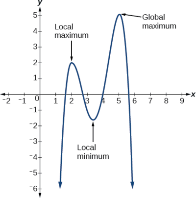
Figure $\PageIndex{25}$: Graph of an even-degree polynomial that denotes the local maximum and minimum and the global maximum.

$QA.png$ Do all polynomial functions have a global minimum or maximum?

No. Only polynomial functions of even degree have a global minimum or maximum. For example, $f(x)=x$ has neither a global maximum nor a global minimum.

Discontinuities

A function has discontinuities at the places where there are breaks in the graph of $f$. Discontinuities take on several different appearances. We classify types of discontinuities as removable discontinuities, infinite discontinuities, or jump discontinuities. Intuitively, a removable discontinuity is a discontinuity for which there is a hole in the graph, a jump discontinuity is a noninfinite discontinuity for which the sections of the function do not meet up, and an infinite discontinuity is a discontinuity located at a vertical asymptote.

Three graphs, each showing a different discontinuity. The first is removable discontinuity. Here, the given function is a line with positive slope. At a point x=a, where a>0, there is an open circle on the line and a closed circle a few units above the line. The second is a jump discontinuity. Here, there are two lines with positive slope. The first line exists for x<=a, and the second exists for x>a, where a>0. The first line ends at a solid circle where x=a, and the second begins a few units up with an open circle at x=a. The third discontinuity type is infinite discontinuity. Here, the function has two parts separated by an asymptote x=a. The first segment is a curve stretching along the x axis to 0 as x goes to negative infinity and along the y axis to infinity as x goes to zero. The second segment is a curve stretching along the y axis to negative infinity as x goes to zero and along the x axis to 0 as x goes to infinity. — Figure $\PageIndex{26}$: Discontinuities are classified as (a) removable, (b) jump, or (c) infinite.

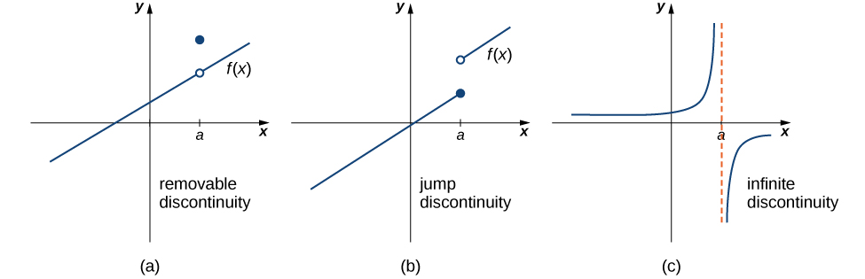
Figure $\PageIndex{26}$ illustrates the differences in these types of discontinuities. Although these terms provide a handy way of describing three common types of discontinuities, keep in mind that not all discontinuities fit neatly into these categories.

a. \(f(x)=5−x+x^3\)	b. \(f(x)=\dfrac{1+4x}{2x−1}\)	c. \(f(x)=\sqrt{4−3x} \)
a. Answer \((−\infty,\infty)\)	b. Answer \((−\infty,\dfrac{1}{2})\cup(\dfrac{1}{2},\infty) \)	c. Answer \( (-\infty,4/3 ] \)

a. Answer Domain: \( (2, 8] \) Range: \( [6, 8) \)	b. Answer Domain: \( (-\infty, 1] \) Range: \( [0,\infty) \)	c. Answer Domain: \( (−\infty,\infty) \) Range: \( (−\infty,\infty) \)
d. Answer Domain: \( (−\infty,0) \cup (0,\infty) \) Range: \( (−\infty,0) \cup (0,\infty) \)	e. Answer Domain: \((−\infty,\infty)\) Range: \( [0,\infty) \)	f. Answer Domain: \((−\infty,\infty)\) Range: \( [0,\infty) \)
g. Answer Domain: \((−\infty,2) \cup (2,\infty) \) Range: \( [-2,-2] \cup [0,\infty) \)	h. Answer Domain: \( (−\infty,\infty) \) Range: \( (−\infty, \infty) \)	i. Answer Domain: \( (−\infty,\infty) \) Range: \( (-\infty, -2] \cup [-1,-1] \cup [0,0] \cup [1,1] \cup [2,\infty) \)

a)	b)	c)
$Graph of a function from \(\left(2, 8\right]\).$	$Graph of a function from (-infinity, 2].$
d) Asymptotes at x=0 and y=0	e)	f) Open circle at (0,2)

g) Open circles at (2,2) and (2,-2)	h) Asymptote at \(x=0,\) filled circle at (0,0)	i) Each horizontal segment ends in an open circle