7.3: Vectors in 2D

Learning Objectives 

• Perform basic vector operations (scalar multiplication, addition, subtraction).
• Express a vector in component form.
• Evaluate the magnitude and direction angle of a vector.
• Express a vector in terms of unit vectors.

When describing the movement of an airplane in flight, it is important to communicate two pieces of information: the direction in which the plane is traveling and the plane’s speed. When measuring a force, such as the thrust of the plane’s engines, it is important to describe not only the strength of that force, but also the direction in which it is applied. Some quantities, such as velocity or force, are defined in terms of both size (also called magnitude) and direction. A quantity that has magnitude and direction is called a vector. In this text, we denote vectors by boldface letters, such as \(\mathbf{v}\). Many times, we will also include an arrow or harpoon above the boldface letter, giving us \(\vec{v}\) or \(\vecs{v}\). This is how we will write vectors by hand, since it's hard to write in boldface.

Definition: Vector

A vector is a quantity that has both magnitude and direction.

Vector Representation

Geometric Perspective

A vector in a plane is represented by a directed line segment (an arrow). The endpoints of the segment are called the initial point and the terminal point of the vector. An arrow from the initial point to the terminal point indicates the direction of the vector. The length of the line segment represents its magnitude. We use the notation \(\|\vecs{v}\|\) to denote the magnitude of the vector \(\vecs{v}\).

Definition: Zero vector

A vector with an initial point and terminal point that are the same is called the zero vector, denoted \(\vecs{0}\). The zero vector is the only vector without a direction, and by convention can be considered to have any direction convenient to the problem at hand.

Vectors with the same magnitude and direction are called equivalent vectors. We treat equivalent vectors as equal, even if they have different initial points. Thus, if \(\vecs{v}\) and \(\vecs{w}\) are equivalent, we write

\(\vecs{v}=\vecs{w}.\)

Definition I: equivalent vectors

Vectors are said to be equivalent vectors if they have the same magnitude and direction.

Figure \(\PageIndex{0}\): (a) A vector is represented by a directed line segment
from its initial point to its terminal point. (b) Vectors \(\vecs{v}_1\) through \(\vecs{v}_5\) are equivalent.

The vectors in Figure \(\PageIndex{0}\) are equivalent. Each vector has the same length and direction. A closely related concept is the idea of parallel vectors. Two vectors are said to be parallel if they have the same or opposite directions. We explore this idea in more detail later in the chapter. A vector is defined by its magnitude and direction, regardless of where its initial point is located.

The use of boldface, lowercase letters to name vectors is a common representation in print, but there are alternative notations. When writing the name of a vector by hand, for example, it is easier to sketch an arrow over the variable to show it is a vector: \(\vec{v}\). When a vector has initial point \(P\) and terminal point \(Q\), the notation \(\vecd{PQ}\) is useful because it indicates the direction and location of the vector.

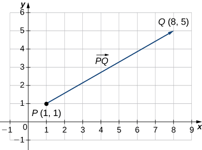
Example \(\PageIndex{1}\): Sketch a Vector

Sketch a vector in the plane from initial point \(P(1,1)\) to terminal point \(Q(8,5)\).

Solution

See Figure \(\PageIndex{1}\). Because the vector goes from point \(P\) to point \(Q\), we name it \(\vecd{PQ}\).

Figure \(\PageIndex{1}\): The vector with initial point \((1,1)\) and terminal point \((8,5)\) is named \(\vecd{PQ}\).

Try It \(\PageIndex{1}\)

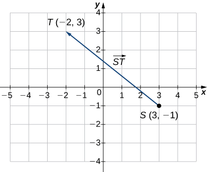
Sketch the vector \(\vecd{ST}\) where \(S\) is point \((3,−1)\) and \(T\) is point \((−2,3).\)

Hint

The first point listed in the name of the vector is the initial point of the vector.

Answer

Working with vectors in a plane is easier when we are working in a coordinate system. When the initial points and terminal points of vectors are given in Cartesian coordinates, computations become straightforward.

Example \(\PageIndex{2}\): Compare Vectors Graphically

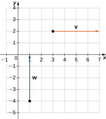
Are \(\vecs{v}\) and \(\vecs{w}\) equivalent vectors?

a.  \(\vecs{v}\) has initial point \((3,2)\) and terminal point \((7,2)\),  \(\vecs{w}\) has initial point \((1,−4)\) and terminal point \((1,0)\).

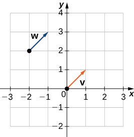
b. \(\vecs{v}\) has initial point \((0,0)\) and terminal point \((1,1)\), \(\vecs{w}\) has initial point \((−2,2)\) and terminal point \((−1,3)\).

Solution

a. The vectors are each \(4\) units long, but they are oriented in different directions. So \(\vecs{v}\) and \(\vecs{w}\) are not equivalent (Figure \(\PageIndex{2a}\)).

Figure \(\PageIndex{2a}\): These vectors are not equivalent.

b. Based on Figure \(\PageIndex{2b}\), and using a bit of geometry, it is clear these vectors have the same length and the same direction, so \(\vecs{v}\) and \(\vecs{w}\) are equivalent.

Figure \(\PageIndex{2b}\): These vectors are equivalent.

Try It \(\PageIndex{2}\)

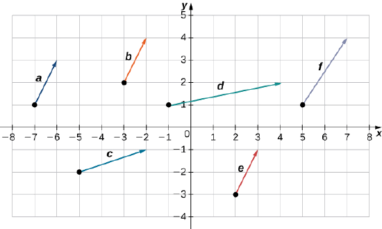
Which of the following vectors are equivalent?

Hint

Equivalent vectors have both the same magnitude and the same direction.

Answer

Vectors \(\vecs{a}, \vecs{b}\), and \(\vecs{e}\) are equivalent.

Algebraic Perspective

Vector Components

Since the location of the initial point of a vector is irrelevant when determining equivalent vectors, knowing the location of the initial and terminal point of a vector is unnecessary. Consequently, working with vectors in a plane can be further simplified by writing them in component form.

Definition: Component Form

Irregardless of the location of its initial point, a vector can be written in component form as

\(\vecs{v}=⟨x,y⟩.\)

The scalars \(x\) and \(y\) are called the components of the vector \(\vecs{v}\). These scalars are measures of the horizontal and vertical distances from the initial point to the terminal point of a vector. The horizontal distance is \(x\) and the vertical distance is \(y\).

We have seen how to plot a vector when we are given an initial point and a terminal point. However, because a vector can be placed anywhere in a plane, it may be easier to perform calculations with a vector when its initial point coincides with the origin. We call a vector with its initial point at the origin a standard-position vector.

Definition: Standard Position Vector

The standard-position vector is the vector with its initial point at the origin. This vector can be written in component form as

\( \vecs{v}=⟨x,y⟩.\) 

Because its initial point is \((0,0)\), the terminal point is of the standard position vector is \((x,y)\) and the scalars \(x\) and \(y\) are the components of \(\vecs{v}\). 

 When writing the component form of a vector, it is important to distinguish between \(⟨x,y⟩\) and \((x,y)\). The first ordered pair uses angle brackets to describe a vector, whereas the second uses parentheses to describe a point in a plane.

When we have a vector not already in standard position, we can determine its component form algebraically using the coordinates of the initial point and the terminal point. To find it algebraically, we subtract the \(x\)-coordinate of the initial point from the \(x\)-coordinate of the terminal point to get the \(x\)-component, and we subtract the \(y\)-coordinate of the initial point from the \(y\)-coordinate of the terminal point to get the \(y\)-component.

Howto: Given an initial and terminal point, find component form.

Let \(\vecs{v}\) be a vector with initial point \(P(x_i,y_i)\) and terminal point \(Q(x_t,y_t)\). Then we can express \(\vecs{v}\) in component form as

\(\vecs{v}=⟨x_t−x_i,y_t−y_i⟩\). 

Because the vector goes from point \(P\) to point \(Q\), it is named \(\vecd{PQ}\).

When we have a vector not already in standard position, we can determine its component form in one of two ways. We can use a geometric approach, in which we sketch the vector in the coordinate plane and then sketch an equivalent standard-position vector, or, we can find it algebraically.

Example \(\PageIndex{3}\): Express a Vector in Component Form Given its Initial and Terminal Points

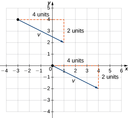
Express vector \(\vecs{v}\) with initial point \((−3,4)\) and terminal point \((1,2)\) in component form.

Solution:

a. Geometric Approach

1. Sketch the vector in the coordinate plane (Figure \(\PageIndex{3a}\)).

2. The terminal point is 4 units to the right and 2 units down from the initial point.

3. Find the point that is 4 units to the right and 2 units down from the origin.

4. In standard position, this vector has initial point \((0,0)\) and terminal point \((4,−2)\). Therefore, its component form is \(\vecs{v}=⟨4,−2⟩.\)

Figure \(\PageIndex{3a}\): These vectors are equivalent.

b. Algebraic Approach

In the first solution, we used a sketch of the vector to see that the terminal point lies 4 units to the right. We can accomplish this algebraically by finding the difference of the \(x\)-coordinates:

\(x_t−x_i=1−(−3)=4.\)

Similarly, the difference of the \(y\)-coordinates shows the vertical length of the vector.

\(y_t−y_i=2−4=−2.\)

So, in component form, \(\vecs{v}=⟨x_t−x_i,y_t−y_i⟩=⟨1−(−3),2−4⟩=⟨4,−2⟩.\)

 Try It  \(\PageIndex{3}\)

Vector \(\vecs{w}\) has initial point \((−4,−5)\) and terminal point \((−1,2)\). Express \(\vecs{w}\) in component form.

Hint

You may use either geometric or algebraic method.

Answer

\(⟨3,7⟩\)

Earlier in this section we stated that two vectors \(\vecs{u}\) and \(\vecs{v}\) are considered equal if they have the same magnitude and the same direction. Another (and much easier) way to show that two vectors are equal is to show that both vectors have the same components.  

Definition II: equivalent vectors

Vectors are equal if they have the same components.

Example \(\PageIndex{4}\): Show Two Vectors Are Equal

Given vector \(\vecs{v}\) with initial point at \((5,−3)\) and terminal point at \((−1,2)\) and vector \(\vecs{u}\) with initial point at \((−1,−3)\) and terminal point at \((−7,2)\),

a. Show the vectors are equal

b. Draw on the same grid:  \(\vecs{v}\) and \(\vecs{u}\) and their position vector.

Solution

Figure \(\PageIndex{4}\)

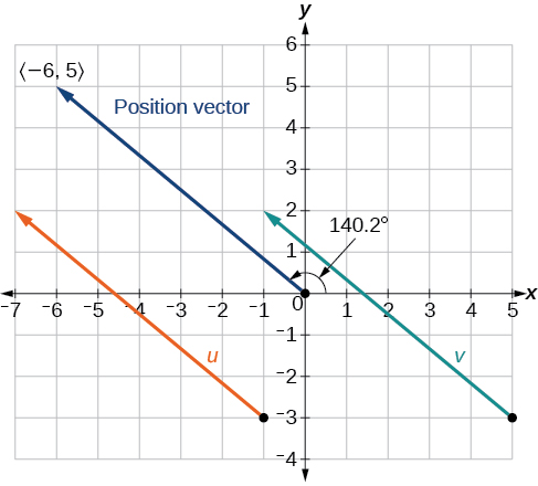
a. The vectors are equal if they have the same components.

\[\begin{align*} \vecs{v} &= ⟨−1−5,2−(−3)⟩  &= ⟨−6,5⟩ \\[4pt] \vecs{u}&= ⟨−7−(−1),2−(−3)⟩  & =⟨−6,5⟩ \end{align*}\]

Since the components of both vectors are the same, \(\vecs{v}\) and \(\vecs{u}\) are the same. Furthermore, their position vector is the same.

b. As shown in Figure \(\PageIndex{4}\), draw the vector \(\vecs{v}\) starting at initial \((5,−3)\) and terminal point \((−1,2)\). Draw the vector \(\vecs{u}\) with initial point \((−1,−3)\) and terminal point \((−7,2)\). The position vector \( ⟨−6,5⟩ \) is the same for both vectors. Furthermore, notice the coordinates of the terminal point of the position vector \( (-6, \; 5) \), are the same as its components.

Combining Vectors

Vectors have many real-life applications, including situations involving force or velocity. For example, consider the forces acting on a boat crossing a river. The boat’s motor generates a force in one direction, and the current of the river generates a force in another direction. Both forces are vectors. We must take both the magnitude and direction of each force into account if we want to know where the boat will go.

A second example that involves vectors is a quarterback throwing a football. The quarterback does not throw the ball parallel to the ground; instead, he aims up into the air. The velocity of his throw can be represented by a vector. If we know how hard he throws the ball (magnitude—in this case, speed), and the angle (direction), we can tell how far the ball will travel down the field.

Geometric Approach

Scalar Multiplication

A real number is often called a scalar in mathematics and physics. Unlike vectors, scalars are generally considered to have a magnitude only, but no direction. Multiplying a vector by a scalar changes the vector’s magnitude. This is called scalar multiplication. Note that changing the magnitude of a vector does not indicate a change in its direction. For example, wind blowing from north to south might increase or decrease in speed while maintaining its direction from north to south.

Definition: Scalar Multiplication

The product \(k\vecs{v}\) of a vector \(\vecs{v}\) and a scalar \(k\) is a vector with a magnitude that is \(|k|\) times the magnitude of \(\vecs{v}\), and with a direction that is the same as the direction of \(\vecs{v}\) if \(k>0\), and opposite the direction of \(\vecs{v}\) if \(k<0\). This is called scalar multiplication. If \(k=0\) or \(\vecs{v}=\vecs{0}\), then \(k\vecs{v}=\vecs{0}.\)

As you might expect, if \(k=−1\), we denote the product \(k\vecs{v}\) as

\(k\vecs{v}=(−1)\vecs{v}=−\vecs{v}.\)

Note that \(−\vecs{v}\) has the same magnitude as \(\vecs{v}\), but has the opposite direction (Figure \(\PageIndex{5.01}\)).

Figure \(\PageIndex{5.01}\): (a) The original vector \( \vecs{v}\) has length \(n\) units. (b) The length of \(2 \vecs{v}\) equals \(2n\) units.
(c) The length of \( \vecs{v}/2\) is \(n/2\) units. (d) The vectors \(\vecs{v}\) and \(−\vecs{v}\) have the same length but opposite directions.

Vector Addition

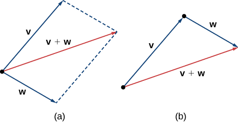
Another operation we can perform on vectors is to add them together in vector addition, but because each vector may have its own direction, the process is different from adding two numbers. The most common graphical method for adding two vectors is to place the initial point of the second vector at the terminal point of the first, as in Figure \(\PageIndex{5.02 (a)}\). To see why this makes sense, suppose, for example, that both vectors represent displacement. If an object moves first from the initial point to the terminal point of vector \(\vecs{v}\), then from the initial point to the terminal point of vector \(\vecs{w}\), the overall displacement is the same as if the object had made just one movement from the initial point to the terminal point of the vector \(\vecs{v}+\vecs{w}\). For obvious reasons, this approach is called the triangle method. Notice that if we had switched the order, so that \(\vecs{w}\) was our first vector and \(\vecs{v}\) was our second vector, we would have ended up in the same place. (Again, see Figure \(\PageIndex{5.02 (a)}\).) Thus,

\( \vecs{v}+ \vecs{w}= \vecs{w}+ \vecs{v}.\)

A second method for adding vectors is called the parallelogram method. With this method, we place the two vectors so they have the same initial point, and then we draw a parallelogram with the vectors as two adjacent sides, as in Figure \(\PageIndex{5.02 (b)}\). The length of the diagonal of the parallelogram is the sum. Comparing Figure \(\PageIndex{5.02 (b)}\) and Figure \(\PageIndex{5.02 (a)}\), we can see that we get the same answer using either method. The vector \( \vecs{v}+ \vecs{w}\) is called the vector sum.

Definition: Vector Addition

The sum of two vectors \(\vecs{v}\) and \(\vecs{w}\) can be constructed graphically by placing the initial point of \(\vecs{w}\) at the terminal point of \(\vecs{v}\). Then, the vector sum, \(\vecs{v}+\vecs{w}\), is the vector with an initial point that coincides with the initial point of \(\vecs{v}\) and has a terminal point that coincides with the terminal point of \(\vecs{w}\). This operation is known as vector addition.

Figure \(\PageIndex{5.02}\): (a) When adding vectors by the triangle method, the initial point of \(\vecs{w}\) is the terminal point of \(\vecs{v}\).
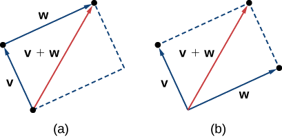
\( \qquad \qquad \) (b) When adding vectors by the parallelogram method, the vectors\(\vecs{v}\) and \(\vecs{w}\) have the same initial point.

Vector Subtraction

It is also appropriate here to discuss vector subtraction. We define \(\vecs{v}−\vecs{w}\) as \(\vecs{v}+(−\vecs{w})=\vecs{v}+(−1)\vecs{w}\). The vector \(\vecs{v}−\vecs{w}\) is called the vector difference. Graphically, the vector \(\vecs{v}−\vecs{w}\) is depicted by drawing a vector from the terminal point of \(\vecs{w}\) to the terminal point of \(\vecs{v}\) (Figure \(\PageIndex{5.03}\)).

Figure \(\PageIndex{5.03}\): (a) The vector difference \(\vecs{v}−\vecs{w}\) is depicted by drawing a vector from the terminal point
of \(\vecs{w}\) to the terminal point of \(\vecs{v}\). (b) The vector\(\vecs{v}−\vecs{w}\) is equivalent to the vector \(\vecs{v}+(−\vecs{w})\).

Example \(\PageIndex{5}\): Perform Vector Operations Graphically

Figure \(\PageIndex{5}\): Vectors \(\vecs{v}\) and \(\vecs{w}\) lie in the same plane.

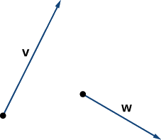
Given the vectors \(v\) and \(w\) shown in Figure \(\PageIndex{5}\), sketch the vectors

1. \(3\vecs{w}\)
2. \(\vecs{v}+\vecs{w}\)
3. \(2\vecs{v}−\vecs{w}\)

 

Solution

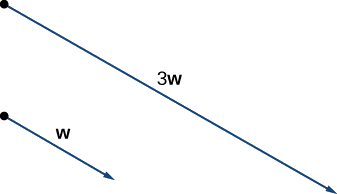
a. The vector \(3\vecs{w}\) has the same direction as \(\vecs{w}\);
it is three times as long as \(\vecs{w}\).

b. Use either addition method to find \(\vecs{v}+\vecs{w}\).

Figure \(\PageIndex{5b}\): To find \(\vecs{v}+\vecs{w}\), align the vectors at their initial points or place the initial point of one vector at the terminal point of the other. (a) The vector\(\vecs{v}+\vecs{w}\) is the diagonal of the parallelogram with sides \(\vecs{v}\) and \(\vecs{w}\). (b) The vector \(\vecs{v}+\vecs{w}\) is the third side of a triangle formed with \(\vecs{w}\) placed at the terminal point of \(\vecs{v}\).

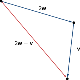
c. 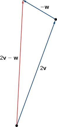To find \(2\vecs{v}−\vecs{w}\), 

First rewrite the expression as \(2\vecs{v}+(−\vecs{w})\).

Then draw the vector \(−\vecs{w}\),

Then add it to the vector \(2\vecs{v}\).

 

 

 

Try It \(\PageIndex{5}\)

Using vectors \(\vecs{v}\) and \(\vecs{w}\) from Example \(\PageIndex{5}\), sketch the vector \(2\vecs{w}−\vecs{v}\).

Hint

First sketch vectors \(2\vecs{w}\) and \(−\vecs{v}\).

Answer

Algebraic Approach

We have defined scalar multiplication and vector addition geometrically. Expressing vectors in component form allows us to perform these same operations algebraically.

Definition: Scalar multiplication and Vector addition

Let \(\vecs{v}=⟨x_1,y_1⟩\) and \(\vecs{w}=⟨x_2,y_2⟩\) be vectors, and let \(k\) be a scalar.

• Scalar multiplication: \( \quad k\vecs{v}=⟨kx_1,ky_1⟩\)
• Vector addition: \( \quad \qquad \vecs{v}+\vecs{w}=⟨x_1,y_1⟩+⟨x_2,y_2⟩=⟨x_1+x_2,y_1+y_2⟩\)

Example \(\PageIndex{6}\): Perform Vector Operations Algebraically

Let \(\vecs{v}\) be the vector with initial point \((2,5)\) and terminal point \((8,13)\), and let \(\vecs{w}=⟨−2,4⟩\).

1. Express \(\vecs{v}\) in component form. Then, using algebra, find
2. \(\vecs{v}+\vecs{w}\),
3. \(3\vecs{v}\), and
4. \(\vecs{v}−2\vecs{w}\).

Solution

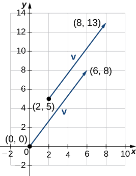a. To place the initial point of \(\vecs{v}\) at the origin, we must translate the vector 2 units to the left and 5 units down (see illustration ton the right). Using the algebraic method, we can express \(\vecs{v}\) as \(\vecs{v}=⟨8−2,13−5⟩=⟨6,8⟩\).

b. To find \(\vecs{v}+\vecs{w}\), add the \(x\)-components and the \(y\)-components separately:

\(\vecs{v}+\vecs{w}=⟨6,8⟩+⟨−2,4⟩=⟨4,12⟩.\)

c. To find \(3\vecs{v}\), multiply \(\vecs{v}\) by the scalar \(k=3\):

\(3\vecs{v}=3⋅⟨6,8⟩=⟨3⋅6,3⋅8⟩=⟨18,24⟩.\)

d. To find \(\vecs{v}−2\vecs{w}\), find \(−2\vecs{w}\) and add it to \(\vecs{v}:\)

\(\vecs{v}−2\vecs{w}=⟨6,8⟩−2⋅⟨−2,4⟩=⟨6,8⟩+⟨4,−8⟩=⟨10,0⟩.\)

Try It \(\PageIndex{6}\)

Let \(\vecs{a}=⟨7,1⟩\) and let \(\vecs{b}\) be the vector with initial point \((3,2)\) and terminal point \((−1,−1).\)

1. Express \(\vecs{b}\) in component form.
2. Find \(3\vecs{a}−4\vecs{b}.\)

Hint To find \(3\vecs{a}−4\vecs{b}\), start by finding the scalar multiples \(3\vecs{a}\) and \(−4\vecs{b}\).

Answer a \(\vecs{b}=⟨−4,−3⟩\)

Answer b \(3\vecs{a}−4\vecs{b}=⟨37,15⟩\)

Vector Magnitude and Direction

To find the magnitude of a vector, we calculate the distance between its initial point and its terminal point. The magnitude of vector \(\vecs{v}=⟨x,y⟩\) is denoted \(\|\vecs{v}\|,\) or \(|\vecs{v}|\), and can be computed using the formula

\(  \|\vecs{v}\|=\sqrt{x^2+y^2}.\)

Note that because this vector is written in component form, it is equivalent to a vector in standard position, with its initial point at the origin and terminal point \((x,y)\). Thus, it suffices to calculate the magnitude of the vector in standard position. Using the distance formula to calculate the distance between initial point \((0,0)\) and terminal point \((x,y)\), we have

\(  \|\vecs{v}\|=\sqrt{(x−0)^2+(y−0)^2}=\sqrt{x^2+y^2}.\)

Based on this formula, it is clear that for any vector \(\vecs{v}, \|\vecs{v}\|≥0,\) and \(\|\vecs{v}\|=0\) if and only if \(\vecs{v}=\vecs{0}\).

The magnitude of a vector can also be derived using the Pythagorean theorem, as in the following figure.

If you use the components of a vector to define a right triangle,
the magnitude of the vector is the length of the triangle’s hypotenuse.

Magnitude and Direction

Howto: Given a vector in component form, find its magnitude and direction angle.

Figure \(\PageIndex{7.01}\) Illustration of a vector's
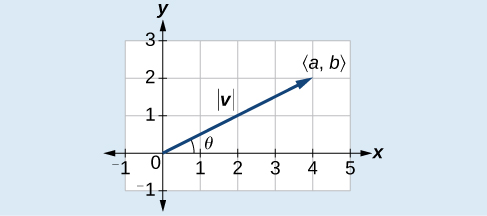
Magnitude \( \|\vecs{v}\| \) and Direction Angle \( \theta \)

Given a vector \( \vecs{v} =⟨a,b⟩\), the magnitude is found by \( \|\vecs{v}\| =\sqrt{a^2+b^2}\).

The direction angle is the positive angle formed between with the positive \(x\)-axis and a vector in standard position. (In other words, place the initial point of the vector at the origin of a coordinate system where the positive \(x\)-axis is horizontal and extends to the right).

The direction angle is found by first finding \(\tan \theta=\left(\dfrac{b}{a}\right)⇒\theta={\tan}^{−1}\left(\dfrac{b}{a}\right)\), as illustrated in Figure \(\PageIndex{7.01}\), and then adjusting the angle if the vector is not in Quadrant I. If the vector is in Quadrant II or Quadrant III, add \(180°\). If the vector is in Quadrant IV, add \(360°\). 

Magnitude and Direction Angle 

Example \(\PageIndex{7a}\): Find the Magnitude and Direction Angle of a Vector

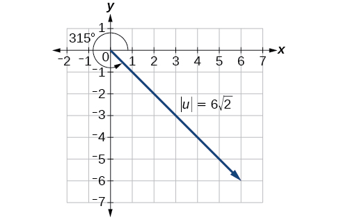
Find the magnitude and direction of the vector with initial point \(P(−8,1)\) and terminal point \(Q(−2,−5)\). Draw the vector.

Solution

Figure \(\PageIndex{7}\)

First, find the position vector \( \vecs{u} \) for \( \vecd{PQ} \).

\[\begin{align*}  \vecs{u} &= ⟨−2,−(−8),−5−1⟩ = ⟨6,−6⟩ \end{align*}\]

We use the Pythagorean Theorem to find the magnitude.

\[\begin{align*}  \|\vecs{u}\| &= \sqrt{{(6)}^2+{(−6)}^2} = \sqrt{72} =6 \sqrt{2} \end{align*}\]

The direction angle is given as

\[\begin{align*} \tan \theta & =\dfrac{−6}{6}=−1\rightarrow \theta={\tan}^{−1}(−1) = −45° \end{align*}\]

However, the angle terminates in the fourth quadrant, so we add \(360°\) to obtain a positive angle. Thus, \(−45°+360°=315°\). See Figure \(\PageIndex{7}\).

Example \(\PageIndex{7b}\) 

Find the magnitude and direction of vector \(\vecs{v}\) with initial point at \((2, -7)\) and terminal point at \((−3, −4)\)

Solution

First, find the position vector \( \vecs{v} \).

\[\begin{align*}  \vecs{v} &= ⟨−3 −2,−4−(−7)⟩ = ⟨−5, 3⟩ \end{align*}\]

We use the Pythagorean Theorem to find the magnitude.

\[\begin{align*}  \|\vecs{v}\| &= \sqrt{{(−5)}^2+3^2} = \sqrt{34}  \end{align*}\]

The direction angle is given as

\[\begin{align*} \tan \theta & =\dfrac{3}{−5} = -0.6.\rightarrow \theta={\tan}^{−1}(-0.6) \approx −31.0° \end{align*}\]

However, the angle terminates in the second quadrant, so we add \(180°\) to obtain correct angle. Thus, the direction angle is \(−31.0°+180°=149.0°\). 

Example \(\PageIndex{7c}\)

Let \(\vecs{v}\) be the vector with initial point \((2,5)\) and terminal point \((8,13)\). Express \(\vecs{v}\) in component form and find \( \| \vecs{v} \| \) and its direction angle. 

Solution

Using the algebraic method, we can express \(\vecs{v}\) as \(\vecs{v}=⟨8−2,13−5⟩=⟨6,8⟩\). The magnitude of \( \vecs{v} \) is:

\(\|\vecs{v}\|=\sqrt{6^2+8^2}=\sqrt{36+64}=\sqrt{100}=10\).

The vector \(\vecs{v}\) is in Quadrant I so the direction angle is

\( \tan \theta = \dfrac{6}{8}⇒\theta={\tan}^{−1}\left(\dfrac{6}{8}\right)  = 36.9° \)

Try It \(\PageIndex{7}\)

Let \(\vecs{a}=⟨−7,−1⟩\). Find \(\|\vecs{a}\|\) and the direction angle (to the nearest tenth of a degree) for \( \vecs{a} \).

Hint

Use the Pythagorean Theorem to find \( \| \vecs{a} \| \). The vector \( \vecs{v} \) is in Quadrant III.

Answer 

\(\|\vecs{a}\| =5\sqrt{2}\). The direction angle is \( 188.1° \)

Find the component form of the vector

\( \;\; \) Figure \(\PageIndex{8.0}\): The components of a vector form the
\( \;\; \) legs of a right triangle, with the vector as the hypotenuse.
_________________________________________________

We have found the components of a vector given its initial and terminal points. In some cases, we may only have the magnitude and direction of a vector, not the points. For these vectors, we can identify the horizontal and vertical components using trigonometry (Figure \(\PageIndex{8.0}\)).

Consider the angle \(θ\) formed by the vector \(\vecs{v}\) and the positive \(x\)-axis. We can see from the triangle that the component form of vector \(\vecs{v}\) is \(⟨\|\vecs{v}\| \cos{θ}, \, \|\vecs{v}\| \sin {θ}⟩\). Therefore, given an angle and the magnitude of a vector, we can use the cosine and sine of the angle to find the components of the vector.

How to: Construct the component form of the vector given its magnitude and direction.

Given vector \(\vecs{v} \) with magnitude \( \| \vecs{v} \| \) and direction angle \( \theta \), the positive angle the vector makes with the positive \(x\)-axis. Then we can express \(\vecs{v}\) in component form as

\(\vecs{v}=⟨ \| \vecs{v} \| \cos \theta, \| \vecs{v} \| \sin \theta ⟩\). 

Example \(\PageIndex{8}\): Express a Vector in Component Form Given Its Magnitude and Direction

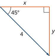Find the component form of a vector with magnitude 4
that forms an angle of \(−45°\) with the \(x\)-axis.

Solution

Let \(x\) and \(y\) represent the components of the vector (see the Figure on the right).
Then \(x=4 \cos(−45°)=2 \sqrt{2}\) and \(y=4 \sin(−45°) \) = \(−2\sqrt{2}\).
The component form of the vector is \(⟨2\sqrt{2},−2\sqrt{2}⟩\).

 Try It \(\PageIndex{8}\)

Find the component form of vector \(\vecs{v}\) with magnitude 10 that forms an angle of \(120°\) with the positive \(x\)-axis.

Hint \(x=\|\vecs{v}\| \cos θ\) and \(y=\|\vecs{v}\| \sin θ\)

Answer \(v=⟨−5,5\sqrt{3}⟩\)

Unit Vectors

Notice that \(\|k\vecs{v}\| =|k|⋅\|\vecs{v}\| \). This is because, if given any nonzero vector \(\vecs{v} = <a, b> \), then a scalar multiple of  \(\vecs{v}\) can be written  \( k \vecs{v}\) or  \(<ka, kb>\). The magnitude of \(\vecs{v}\) is \( \sqrt{ a^2+b^2} \). The corresponding magnitude of the scalar multiple of \(\vecs{v}\) is \( \sqrt{k^2 a^2 + k^2 b^2}\) which can be rewritten as \( k\sqrt{ a^2+b^2}\) or \( \| k \vecs{v} \| \).

Unit vector \(\vecs{u} \) in the direction of \(\vecs{v}\).

 

If we define a vector \(\vecs{u}=\dfrac{1}{\|\vecs{v}\| }\vecs{v}\), it follows that \(\|\vecs{u}\| =\dfrac{1}{\|\vecs{v}\| }(\|\vecs{v}\| )=1\) and we say that \(\vecs{u}\) is the unit vector in the direction of \(\vecs{v}\) (see Figure on the right).

Definition: Unit Vector

The unit vector for any nonzero vector \(\vecs{v}\) is a vector that is in the same direction as \(\vecs{v}\) but with a magnitude of 1.

The unit vector for \(\vecs{v}\) is denoted \( \hat{ \mathbf{v}} \) and is obtained by multiplying a vector by the reciprocal of its magnitude: 

\( \hat{ \mathbf{v}}=\dfrac{1}{\|\vecs{v}\|} \vecs{v}.\)

The process of using scalar multiplication to find a unit vector with a given direction is called normalization.

Example \(\PageIndex{9}\): Find a Unit Vector

Let \(\vecs{v}=⟨1,2⟩\).

1. Find a unit vector with the same direction as \(\vecs{v}\).
2. Find a vector \(\vecs{w}\) with the same direction as \(\vecs{v}\) such that \(\|\vecs{w}\|=7\).

Solution:

a. First, find the magnitude of \(\vecs{v}\), then divide the components of \(\vecs{v}\) by the magnitude:

\[\|\vecs{v}\|=\sqrt{1^2+2^2}=\sqrt{1+4}=\sqrt{5} \nonumber\]

\[\vecs{u}=\dfrac{1}{\|\vecs{v}\|}v=\dfrac{1}{\sqrt{5}}⟨1,2⟩=\left \langle \dfrac{1}{\sqrt{5}},\dfrac{2}{\sqrt{5}}\right \rangle =\left \langle \dfrac{\sqrt{5}}{5},\dfrac{2\sqrt{5}}{5} \right \rangle \nonumber.\]

b. The vector \(\vecs{u}\) is in the same direction as \(\vecs{v}\) and \(\|\vecs{u}\|=1\). Use scalar multiplication to increase the length of \(\vecs{u}\) without changing direction:

\[\vecs{w}=7\vecs{u}=7\left \langle\dfrac{1}{\sqrt{5}},\dfrac{2}{\sqrt{5}}\right \rangle =\left \langle\dfrac{7}{\sqrt{5}},\dfrac{14}{\sqrt{5}}\right \rangle =\left \langle\dfrac{7\sqrt{5}}{5},\dfrac{14\sqrt{5}}{5}\right \rangle \nonumber.\]

 Try It \(\PageIndex{9}\)

Let \(\vecs{v}=⟨9,2⟩\). Find a vector with magnitude \(5\) in the opposite direction as \(\vecs{v}\). Then negate it.

Hint First, find a unit vector in the same direction as \(\vecs{v}\).

Answer \(⟨−\dfrac{45}{\sqrt{85}},−\dfrac{10}{\sqrt{85}}⟩ =⟨−\dfrac{9\sqrt{85}}{17},−\dfrac{2\sqrt{85}}{17}⟩ \)

Standard Unit Vectors

Figure \(\PageIndex{10.0}\): \( v = v_1 + v_2 \)

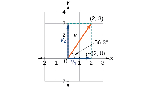
In some applications involving vectors, it is helpful for us to be able to break a vector down into its components. Recall that vectors are comprised of two components: the horizontal component is the \(x\) direction, and the vertical component is the \(y\) direction. For example, we can see in the graph in Figure \(\PageIndex{13}\) that the position vector \(⟨2,3⟩\) comes from adding the vectors \vecs{v_1} and \(\vecs{v_2}\). We have \(\vecs{v_2}\) with initial point \((0,0)\) and terminal point \((2,0)\).

\[\begin{align*} \vecs{v_1} &= ⟨2−0,0−0⟩ = ⟨2,0⟩ \end{align*}\]

We also have \(\vecs{v_2}\) with initial point \((0,0)\) and terminal point \((0, 3)\).

\[\begin{align*} \vecs{v_2} &= ⟨0−0,3−0⟩ = ⟨0,3⟩ \end{align*}\]

Therefore, the position vector is \( \quad \; \vecs{v} = \vecs{v_1} + \vecs{v_2} = ⟨2+0,0+3⟩ = ⟨2,3⟩ \)

Example \(\PageIndex{10}\): Write a Vector as a Sum of Vectors

Write the vector \(\vec{v}\) with initial point \((3,2)\) and terminal point \((7,4)\) as a sum of a horizontal and a vertical vector.

Solution

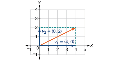First find the standard position.

\[\begin{align*} v &= ⟨7−3,4−2⟩ \\[4pt] &= ⟨4,2⟩ \end{align*}\]

See the illustration on the right.

The horizontal component is \(\vec{v_1}=⟨4,0⟩\) and the vertical component is \(\vec{v_2}=⟨0,2⟩\).

 We have seen how convenient it can be to write a vector in component form. Sometimes, though, it is more convenient to write a vector as a sum of a horizontal vector and a vertical vector. To make this easier, let’s look at standard unit vectors.

Definition: Standard Unit Vectors

    Standard unit vectors \(\hat{\mathbf i}\) and \(\hat{\mathbf j}\)

The standard unit vectors are the vectors \(\hat{\mathbf i}=⟨1,0⟩\) and \(\hat{\mathbf j}=⟨0,1⟩\)

Vector \(\hat{\mathbf i}\) is the horizontal unit vector with a magnitude 1.
Vector \(\hat{\mathbf j}\) is the vertical unit vector with a magnitude 1.

Any vector in component form can be expressed as a sum of the standard unit vectors (called standard unit vector form):

\( \vecs{v} = <a, b> = a \hat{\mathbf i}+ b \hat{\mathbf j} \)

By applying the properties of vectors, it is possible to express any vector in terms of \(\hat{\mathbf i}\) and \(\hat{\mathbf j}\) in what we call a linear combination:

\( \vecs{v}=⟨x,y⟩=⟨x,0⟩+⟨0,y⟩=x⟨1,0⟩+y⟨0,1⟩=x\hat{\mathbf i}+y\hat{\mathbf j}. \)

Thus, \(\vecs{v}\) is the sum of a horizontal vector with magnitude \(x\), and a vertical vector with magnitude \(y\), as in Figure \(\PageIndex{11b}\).

Figure \(\PageIndex{11b}\): The vector \(\vecs{v}\) is the sum of \(x\hat{\mathbf i}\) and \(y\hat{\mathbf j}\).

Example \(\PageIndex{11}\): Write a Vector in Standard Unit Vector Form

Express the vector \(\vecs{w}=⟨3,−4⟩\) as a sum of the standard unit vectors.

Solution:

\[\vecs{w}=⟨3,−4⟩=3 \hat{\mathbf i}−4 \hat{\mathbf j}. \nonumber\]

 Try It \(\PageIndex{11}\)

Let \(\vecs{a}=⟨16,−11⟩\) Express \(\vecs{a}\) in standard unit vector form.

Answer

\(\vecs{a}=16 \hat{\mathbf i}−11 \hat{\mathbf j}\)

Example \(\PageIndex{12}\): Express a Vector in Standard Unit Vector Form Given its Initial and Terminal Points

Given a vector \(\vecs{v}\) with initial point \(P=(2,−6)\) and terminal point \(Q=(−6,6)\), write the vector in terms of \( \hat{\mathbf i}\) and \(\ \hat{\mathbf j}\).

Solution

\[\begin{align*} \vecs{v} &= (x_Q−x_P)\hat{\mathbf i}+(y_Q−y_P)\hat{\mathbf j} \\[4pt]
&=(−6−2)\hat{\mathbf i}+(6−(−6))\hat{\mathbf j} = −8\hat{\mathbf i}+12\hat{\mathbf j} \end{align*}\]

 Try It \(\PageIndex{12}\)

Write the vector \(\vecs{u}\) with initial point \(P=(−1,6)\) and terminal point \(Q=(7,−5)\) in terms of \( \hat{\mathbf i}\) and \( \hat{\mathbf j}\).

Answer

\( \vecs{u}=8\hat{\mathbf i}−11\hat{\mathbf j}\)

Example \(\PageIndex{13}\): Perform Scalar Multiplication with Vectors written in Standard Unit Vector Form

Given vector \(\vecs{v}=3\hat{\mathbf i}−1\hat{\mathbf j}\), find \(3\vecs{v}\), \(\dfrac{1}{2} \vecs{v}\), and \(−\vecs{v}\).

Solution

\[\begin{align*} 3\vecs{v} &= 3⋅( 3\hat{\mathbf i}−1\hat{\mathbf j})  = 9\hat{\mathbf i}−3\hat{\mathbf j} \\[4pt]
\dfrac{1}{2}\vecs{v} &= \dfrac{1}{2}⋅( 3\hat{\mathbf i}−1\hat{\mathbf j})  =\dfrac{3}{2} \hat{\mathbf i} − \dfrac{1}{2} \hat{\mathbf j} \\[4pt]
−\vecs{v} &= −( 3\hat{\mathbf i}−1\hat{\mathbf j})  =−3\hat{\mathbf i}+1\hat{\mathbf j}
\end{align*}\]

 Try It \(\PageIndex{13}\)

Find the scalar multiple \(3 \vecs{u}\) given \(\vecs{u}=5\hat{\mathbf i}+4\hat{\mathbf j} \).

Answer

\(3\vecs{u} =15\hat{\mathbf i}+12\hat{\mathbf j} \)

Example \(\PageIndex{14}\) Algebraic Operations using Vectors Written in Standard Unit Vector Form 

Given \(\vecs{u}=3\hat{\mathbf i}−2\hat{\mathbf j}\) and \(\vecs{v}=−\hat{\mathbf i}+4\hat{\mathbf j} \), find new vectors \( \vecs{w_1}=3\vecs{u}+2\vecs{v}\) and  \( \vecs{w_2}=\vecs{u}−\vecs{v}\).

Solution

First, we must multiply each vector by the scalar.

\[\begin{align*} 3\vecs{u} &= 3(3\hat{\mathbf i}−2\hat{\mathbf j})  = 9\hat{\mathbf i}−6\hat{\mathbf j} \\[4pt]
2\vecs{v} &= 2(−\hat{\mathbf i}+4\hat{\mathbf j})  = −2\hat{\mathbf i}+8\hat{\mathbf j} \end{align*}\]

Then, add the two together.

\[\begin{align*} \vecs{w_1} &= 3\vecs{u}+2\vecs{v} \\[4pt]
&=(9\hat{\mathbf i}−6\hat{\mathbf j}) +  (−2\hat{\mathbf i}+8\hat{\mathbf j}) \\[4pt]
&= (9−2)\hat{\mathbf i} +(−6+8)\hat{\mathbf j} = 7\hat{\mathbf i}+2\hat{\mathbf j} \end{align*}\]

To find the difference of two vectors, add the negative components of \(\vecs{v}\) to \(\vecs{u}\). Thus,

\[\begin{align*} \vecs{w_2} &= \vecs{u}−\vecs{v} \\[4pt]
&=(3\hat{\mathbf i}−2\hat{\mathbf j}) + (− (−\hat{\mathbf i}+4\hat{\mathbf j}) ) \\[4pt]
&=3\hat{\mathbf i}−2\hat{\mathbf j} + \hat{\mathbf i}−4\hat{\mathbf j} \\[4pt]
&= (9+1)\hat{\mathbf i} +(−2−4)\hat{\mathbf j} = 10\hat{\mathbf i}−6\hat{\mathbf j} \end{align*}\]

 Try It  \(\PageIndex{14}\)

Given \(\vecs{u}=3\hat{\mathbf i}−2\hat{\mathbf j}\),  \(\vecs{v}=−\hat{\mathbf i}+ 4\hat{\mathbf j}\), \(\vecs{v_1}=2\hat{\mathbf i}−3\hat{\mathbf j}\) and \(\vecs{v_2}=4\hat{\mathbf i}+5\hat{\mathbf j}\), find vectors \( \vecs{u}+\vecs{v} \),  \( \vecs{u}−\vecs{v} \) and \( 2\vecs{v_1}−3\vecs{v_2} \).

Answer

\[ \begin{align*}
  \vecs{u}+\vecs{v} &= 2\hat{\mathbf i} + 2\hat{\mathbf j} \\[4pt]
  \vecs{u}−\vecs{v} &= 4\hat{\mathbf i} − 6\hat{\mathbf j} \\[4pt]
  2\vecs{v_1}−3\vecs{v_2} &= −8\hat{\mathbf i} −21\hat{\mathbf j}
\end{align*} \]

Example \(\PageIndex{15}\): Construct a Vector Given Its Magnitude and Direction

Write a vector in standard unit vector notation that has a length of \(7\) and makes an angle of \(135°\) with the positive x-axis.

Solution

Using the conversion formulas \(x=\| \vecs{v} \| \cos\theta \hat{\mathbf i}\) and \(y=\| \vecs{v} \| \sin \theta \hat{\mathbf j}\), we find that

\[ \begin{align*}
x &= 7\cos(135°)\hat{\mathbf i} = −\dfrac{7\sqrt{2}}{2} \hat{\mathbf i} \\[4pt]
y &=7 \sin(135°)\hat{\mathbf j} = \dfrac{7\sqrt{2}}{2}  \hat{\mathbf j} \end{align*}\]

This vector can be written as \(\vecs{v}=7\cos(135°)\hat{\mathbf i}+7\sin(135°)\hat{\mathbf j}\) which simplified becomes

\(\vecs{v}=−\dfrac{7\sqrt{2}}{2}\hat{\mathbf i}+\dfrac{7\sqrt{2}}{2}\hat{\mathbf j}\)

 Try It \(\PageIndex{15}\)

Let  \(\vecs{b}\) be a unit vector that forms an angle of \(225°\) with the positive \(x\)-axis. Express \(\vecs{b}\) in terms of the standard unit vectors.

Hint

Use sine and cosine to find the components of \(\vecs{b}\).

Answer

\( \vecs{b}=−\dfrac{\sqrt{2}}{2} \hat{\mathbf i}−\dfrac{\sqrt{2}}{2} \hat{\mathbf j}\)

Example \(\PageIndex{16}\): Find the Unit Vector in the Direction of \(\vecs{v}\)

Find a unit vector in the same direction as \(\vecs{v}=−5\hat{\mathbf i} +12\hat{\mathbf j} \).

Solution

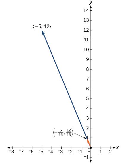First, we will find the magnitude.

\[\begin{align*} \| \vecs{v} \| &= \sqrt{{(−5)}^2+{(12)}^2} = \sqrt{25+144} =\sqrt{169} = 13 \end{align*}\]

Then we divide each component by \(| \vecs{v} |\), which gives a unit vector in the same direction as \(\vec{v}\):

\( \dfrac{1}{ \| \vecs{v} \|} \cdot \vecs{v} = −\dfrac{5}{13}\hat{\mathbf i}+\dfrac{12}{13}\hat{\mathbf j} \)

The figure on the right illustrates vector \( \vecs{v} \) and its corresponding unit vector \( \hat{\mathbf v} \)

Verify that the magnitude of the unit vector equals \(1\). The magnitude of \(−\dfrac{5}{13}\hat{\mathbf i}+\dfrac{12}{13}\hat{\mathbf j}\) is given as

\[\begin{align*} \sqrt{ {\left(−\dfrac{5}{13}\right)}^2+{ \left(\dfrac{12}{13}\right) }^2 } &= \sqrt{\dfrac{25}{169}+\dfrac{144}{169}} \\[4pt] &= \sqrt{\dfrac{169}{169}} = 1 \end{align*}\]

The vector \( \hat{\mathbf u}=\dfrac{5}{13}\hat{\mathbf i}+\dfrac{12}{13}\hat{\mathbf j}\) is a unit vector because it has a magnitude of \(1\). It is in the same direction as \(\vecs{v} \) because it is a positive scalar multiple of \( \vecs{v} \).

 Try It \(\PageIndex{16}\)

A vector travels from the origin to the point \((−3, −5)\). Find the magnitude and direction angle of the vector (exactly and to the nearest hundredth). Write the vector in standard unit vector notation and find the unit vector that goes in the same direction.

Answer

Magnitude = \( \sqrt{34} \approx 5.83  \)

Direction Angle: Vector is in QIII so \( \theta={\tan}^{−1} \left( \dfrac{−5}{−3} \right) + 180° \approx 239.04° \)

\( \vecs{v} =\sqrt{34}\cos(239.04°)\hat{\mathbf i}+\sqrt{34}\sin(239.04°)\hat{\mathbf j} = −3\hat{\mathbf i} −5\hat{\mathbf j} \)

Unit Vector: \(  \hat{\mathbf u} = − \dfrac{3\sqrt{34}}{34}\hat{\mathbf i} − \dfrac{5\sqrt{34}}{34}\hat{\mathbf j}  \)

Applications of Vectors

Because vectors have both direction and magnitude, they are valuable tools for solving problems involving such applications as motion and force. Recall the boat example and the quarterback example we described earlier. Here we look at two other examples in detail.

Example \(\PageIndex{17}\): Finding Resultant Force

Jane’s car is stuck in the mud. Lisa and Jed come along in a truck to help pull her out. They attach one end of a tow strap to the front of the car and the other end to the truck’s trailer hitch, and the truck starts to pull. Meanwhile, Jane and Jed get behind the car and push. The truck generates a horizontal force of 300 lb on the car. Jane and Jed are pushing at a slight upward angle and generate a force of 150 lb on the car. These forces can be represented by vectors, as shown in Figure \(\PageIndex{17}\). The angle between these vectors is 15°. Find the resultant force (the vector sum) and give its magnitude to the nearest tenth of a pound and its direction angle from the positive \(x\)-axis.

Figure \(\PageIndex{17}\): Two forces acting on a car in different directions.

Solution

To find the effect of combining the two forces, add their representative vectors. First, express each vector in component form or in terms of the standard unit vectors. For this purpose, it is easiest if we align one of the vectors with the positive \(x\)-axis. The horizontal vector, then, has initial point \((0,0)\) and terminal point \((300,0)\). It can be expressed as \(⟨300,0⟩\) or \(300 \hat{\mathbf i}\).

The second vector has magnitude \(150\) and makes an angle of \(15°\) with the first, so we can express it as \(⟨150 \cos(15°),150 \sin(15°)⟩,\) or \(150 \cos(15°)\hat{\mathbf i}+150 \sin(15°)\hat{\mathbf j}\). Then, the sum of the vectors, or resultant vector, is \(\vecs{r}=⟨300,0⟩+⟨150 \cos(15°),150 \sin(15°)⟩,\) and we have

\[\|\vecs{r}\|=\sqrt{(300+150 \cos(15°))^2+(150 \sin(15°))^2}≈446.6. \nonumber\]

The angle \(θ\) made by \(\vecs{r}\) and the positive \(x\)-axis has \(\tan θ=\dfrac{150 \sin 15°}{(300+150\cos 15°)}≈0.09\), so \(θ≈ \tan^{−1}(0.09)≈5°\), which means the resultant force \(\vecs{r}\) has an angle of \(5°\) above the horizontal axis.

Example \(\PageIndex{18}\): Finding Resultant Velocity

An airplane flies due west at an airspeed of \(425\) mph. The wind is blowing from the northeast at \(40\) mph. What is the ground speed of the airplane? What is the bearing of the airplane?

Solution

Let’s start by sketching the situation described (Figure \(\PageIndex{18}\)).

Figure \(\PageIndex{18}\): Initially, the plane travels due west. The wind is from the northeast, so it is blowing to the southwest. The angle between the plane’s course and the wind is \(45°\). (Figure not drawn to scale.)

Set up a sketch so that the initial points of the vectors lie at the origin. Then, the plane’s velocity vector is \(\vecs{p}=−425\hat{\mathbf i}\). The vector describing the wind makes an angle of \(225°\) with the positive \(x\)-axis:

\[\vecs{w}=⟨40 \cos(225°),40 \sin(225°)⟩=⟨−\dfrac{40}{\sqrt{2}},−\dfrac{40}{\sqrt{2}}⟩=−\dfrac{40}{\sqrt{2}}\hat{\mathbf i}−\dfrac{40}{\sqrt{2}}\hat{\mathbf j}. \nonumber\]

When the airspeed and the wind act together on the plane, we can add their vectors to find the resultant force:

\[\vecs{p}+\vecs{w}=−425\hat{\mathbf i}+(−\dfrac{40}{\sqrt{2}}\hat{\mathbf i}−\dfrac{40}{\sqrt{2}}\hat{\mathbf j})=(−425−\dfrac{40}{\sqrt{2}})\hat{\mathbf i}−\dfrac{40}{\sqrt{2}}\hat{\mathbf j}. \nonumber\]

The magnitude of the resultant vector shows the effect of the wind on the ground speed of the airplane:

\(\|\vecs{p}+\vecs{w}\|=\sqrt{(−425−\dfrac{40}{\sqrt{2}})^2+(−\dfrac{40}{\sqrt{2}})^2}≈454.17 \, mph\)

As a result of the wind, the plane is traveling at approximately \(454\) mph relative to the ground.

To determine the bearing of the airplane, we want to find the direction of the vector \(\vecs{p}+\vecs{w}\):

\(\tan θ=\dfrac{−\dfrac{40}{\sqrt{2}}}{(−425−\dfrac{40}{\sqrt{2}})}≈0.06\)

\(θ≈3.57°\).

The overall direction of the plane is \(3.57°\) south of west.

Try It \(\PageIndex{18}\)

An airplane flies due north at an airspeed of \(550\) mph. The wind is blowing from the northwest at \(50\) mph. What is the ground speed of the airplane?

Hint

Sketch the vectors with the same initial point and find their sum.

Answer

Approximately \(516\) mph

Key Concepts

• Vectors are used to represent quantities that have both magnitude and direction.
• We can add vectors by using the parallelogram method or the triangle method to find the sum. We can multiply a vector by a scalar to change its length or give it the opposite direction.
• Subtraction of vectors is defined in terms of adding the negative of the vector.
• A vector is written in component form as \(\vecs{v}=⟨x,y⟩\).
• The magnitude of a vector is a scalar: \(‖\vecs{v}‖=\sqrt{x^2+y^2}\).
• A unit vector \(\vecs{u}\) has magnitude \(1\) and can be found by dividing a vector by its magnitude: \(\vecs{u}=\dfrac{1}{‖\vecs{v}‖}\vecs{v}\). The standard unit vectors are \(\hat{\mathbf i}=⟨1,0⟩\) and \(\hat{\mathbf j}=⟨0,1⟩\). A vector \(\vecs{v}=⟨x,y⟩\) can be expressed in terms of the standard unit vectors as \(\vecs{v}=x\hat{\mathbf i}+y\hat{\mathbf j}\).
• Vectors are often used in physics and engineering to represent forces and velocities, among other quantities.

Glossary

component

a scalar that describes either the vertical or horizontal direction of a vector

equivalent vectors

vectors that have the same magnitude and the same direction

initial point

the starting point of a vector

magnitude

the length of a vector

parallelogram method

a method for finding the sum of two vectors; position the vectors so they share the same initial point; the vectors then form two adjacent sides of a parallelogram; the sum of the vectors is the diagonal of that parallelogram

scalar

a real number

scalar multiplication

a vector operation that defines the product of a scalar and a vector

standard-position vector

a vector with initial point \((0,0)\)

standard unit vectors

unit vectors along the coordinate axes: \(\hat{\mathbf i}=⟨1,0⟩,\, \hat{\mathbf j}=⟨0,1⟩\)

terminal point

the endpoint of a vector

triangle method

a method for finding the sum of two vectors; position the vectors so the terminal point of one vector is the initial point of the other; these vectors then form two sides of a triangle; the sum of the vectors is the vector that forms the third side; the initial point of the sum is the initial point of the first vector; the terminal point of the sum is the terminal point of the second vector

unit vector

a vector with magnitude \(1\)

vector

a mathematical object that has both magnitude and direction

vector addition

a vector operation that defines the sum of two vectors

vector difference

the vector difference \(\vecs{v}−\vecs{w}\) is defined as \(\vecs{v}+(−\vecs{w})=\vecs{v}+(−1)\vecs{w}\)

vector sum

the sum of two vectors, \(\vecs{v}\) and \(\vecs{w}\), can be constructed graphically by placing the initial point of \(\vecs{w}\) at the terminal point of \(\vecs{v}\); then the vector sum \(\vecs{v}+\vecs{w}\) is the vector with an initial point that coincides with the initial point of \(\vecs{v}\), and with a terminal point that coincides with the terminal point of \(\vecs{w}\)

zero vector

the vector with both initial point and terminal point \((0,0)\)

Contributors and Attributions

• Gilbert Strang (MIT) and Edwin “Jed” Herman (Harvey Mudd) with many contributing authors. This content by OpenStax is licensed with a CC-BY-SA-NC 4.0 license. Download for free at http://cnx.org.