2.5: Limits at Infinity

We need to know the behavior of $f$ as $x→±∞$. In this section, we define limits at infinity and show how these limits affect the graph of a function.

We begin by examining what it means for a function to have a finite limit at infinity. Then we study the idea of a function with an infinite limit at infinity. Back in Introduction to Functions and Graphs, we looked at vertical asymptotes; in this section we deal with horizontal and oblique asymptotes.

Limits at Infinity and Horizontal Asymptotes

Recall that $\displaystyle \lim_{x→a}f(x)=L$ means $f(x)$ becomes arbitrarily close to $L$ as long as $x$ is sufficiently close to $a$. We can extend this idea to limits at infinity. For example, consider the function $f(x)=2+\frac{1}{x}$. As can be seen graphically in Figure and numerically in Table, as the values of $x$ get larger, the values of $f(x)$ approach $2$. We say the limit as $x$ approaches $∞$ of $f(x)$ is $2$ and write $\displaystyle \lim_{x→∞}f(x)=2$. Similarly, for $x<0$, as the values $|x|$ get larger, the values of $f(x)$ approaches $2$. We say the limit as $x$ approaches $−∞$ of $f(x)$ is $2$ and write $\displaystyle \lim_{x→−∞}f(x)=2$.

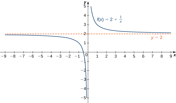
Figure $\PageIndex{1}$:The function approaches the asymptote $y=2$ as $x$ approaches $±∞$.

Values of a function $f$ as $x→±∞$

$x$	10	100	1,000	10,000
$2+\frac{1}{x}$	2.1	2.01	2.001	2.0001
$x$	−10	−100	−1000	−10,000
$2+\frac{1}{x}$	1.9	1.99	1.999	1.9999

More generally, for any function $f$, we say the limit as $x→∞$ of $f(x)$ is $L$ if $f(x)$ becomes arbitrarily close to $L$ as long as $x$ is sufficiently large. In that case, we write $\displaystyle \lim_{x→ −∞ }f(x)=L$. Similarly, we say the limit as $x→−∞$ of $f(x)$ is $L$ if $f(x)$ becomes arbitrarily close to $L$ as long as $x<0$ and $|x|$ is sufficiently large. In that case, we write $\displaystyle \lim_{x→−∞}f(x)=L$. We now look at the definition of a function having a limit at infinity.

Definition: limit at infinity (Informal)

If the values of $f(x)$ become arbitrarily close to $L$ as $x$ becomes sufficiently large, we say the function $f$ has a limit at infinity and write

$$\lim_{x→∞}f(x)=L.$$

If the values of $f(x)$ becomes arbitrarily close to $L$ for $x<0$ as $|x|$ becomes sufficiently large, we say that the function $f$ has a limit at negative infinity and write

$$\lim_{x→-∞}f(x)=L.$$

If the values $f(x)$ are getting arbitrarily close to some finite value $L$ as $x→∞$ or $x→−∞$, the graph of $f$ approaches the line $y=L$. In that case, the line $y=L$ is a horizontal asymptote of $f$ (Figure). For example, for the function $f(x)=\frac{1}{x}$, since $\displaystyle \lim_{x→∞}f(x)=0$, the line $y=0$ is a horizontal asymptote of $f(x)=\frac{1}{x}$.

Definition: horizontal asymptote

If $\displaystyle \lim_{x→∞}f(x)=L$ or $\displaystyle \lim_{x→−∞}f(x)=L$, we say the line $y=L$ is a horizontal asymptote of $f$.

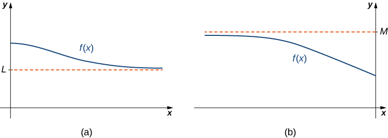
Figure $\PageIndex{2}$: (a) As $x→∞$, the values of $f$ are getting arbitrarily close to $L$. The line $y=L$ is a horizontal asymptote of $f$. (b) As $x→−∞$, the values of $f$ are getting arbitrarily close to $M$. The line $y=M$ is a horizontal asymptote of $f$.

A function cannot cross a vertical asymptote because the graph must approach infinity (or $−∞$) from at least one direction as $x$ approaches the vertical asymptote. However, a function may cross a horizontal asymptote. In fact, a function may cross a horizontal asymptote an unlimited number of times. For example, the function $f(x)=\frac{(cosx)}{x}+1$ shown in Figure intersects the horizontal asymptote $y=1$ an infinite number of times as it oscillates around the asymptote with ever-decreasing amplitude.

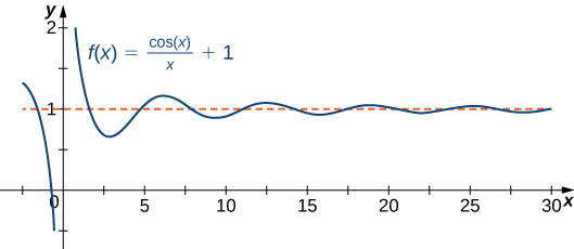
Figure $\PageIndex{3}$: The graph of $f(x)=(cosx)/x+1$ crosses its horizontal asymptote $y=1$ an infinite number of times.

The algebraic limit laws and squeeze theorem we introduced in Introduction to Limits also apply to limits at infinity. We illustrate how to use these laws to compute several limits at infinity.

Example $\PageIndex{1}$: Computing Limits at Infinity

For each of the following functions $f$, valuate $\displaystyle \lim_{x→∞}f(x)$ and $\displaystyle \lim_{x→−∞}f(x)$. Determine the horizontal asymptote(s) for $f$.

1. $f(x)=5−\frac{2}{x^2}$
2. $f(x)=\frac{sinx}{x}$
3. $f(x)=tan^{−1}(x)$

Solution

a. Using the algebraic limit laws, we have

$\displaystyle \lim_{x→∞}(5−\frac{2}{x^2})=\displaystyle \lim_{x→∞}5−2(\displaystyle \lim_{x→∞}\frac{1}{x}).(\displaystyle \lim_{x→∞}\frac{1}{x})$=5−2⋅0=5.

Similarly, $\displaystyle \lim_{x→-∞}f(x)=5$. Therefore, $f(x)=\frac{5−2}{x^2}$ has a horizontal asymptote of $y=5$ and $f$ approaches this horizontal asymptote as $x→±∞$ as shown in the following graph.

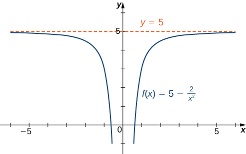
Figure $\PageIndex{4}$: This function approaches a horizontal asymptote as $x→±∞.$

b. Since $-1≤sinx≤1$ for all positive $x$, we have

$\frac{−1}{x}≤\frac{sinx}{x}≤\frac{1}{x}$

for all $x≠0$. Also, since

$\displaystyle \lim_{x→∞}\frac{−1}{x}=0= \displaystyle \lim_{x→∞}\frac{1}{x}$,

we can apply the squeeze theorem to conclude that

$\displaystyle \lim_{x→∞}\frac{sinx}{x}=0.$

Similarly,

$\displaystyle \lim_{x→−∞}\frac{sinx}{x}=0.$

Thus, $f(x)=\frac{sinx}{x}$ has a horizontal asymptote of $y=0$ and $f(x)$ approaches this horizontal asymptote as $x→±∞$ as shown in the following graph.

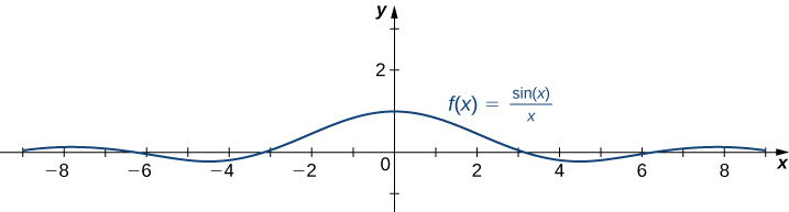
Figure $\PageIndex{5}$: This function crosses its horizontal asymptote multiple times.

c. To evaluate $\displaystyle \lim_{x→∞}tan^{−1}(x)$ and $\displaystyle \lim_{x→−∞}tan^{−1}(x)$, we first consider the graph of $y=tan(x)$ over the interval $(−π/2,π/2)$ as shown in the following graph.

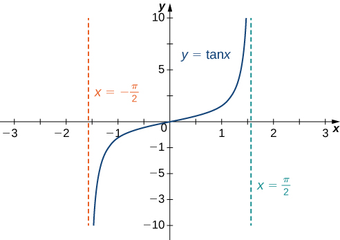
Figure $\PageIndex{6}$: The graph of $tanx$ has vertical asymptotes at $x=±\frac{π}{2}$

Since

$\displaystyle \lim_{x→(π/2)−}tanx=∞,$

it follows that

$\displaystyle \lim_{x→∞}tan^{−1}(x)=\frac{π}{2}.$

Similarly, since

$\displaystyle \lim_{x→(-π/2)^+}tanx=−∞,$

it follows that

$\displaystyle \lim_{x→−∞}tan^{−1}(x)=−\frac{π}{2}.$

As a result, $y=\frac{π}{2}$ and $y=−\frac{π}{2}$ are horizontal asymptotes of $f(x)=tan^{−1}(x)$ as shown in the following graph.

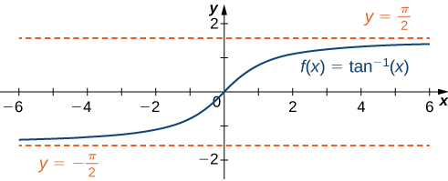
Figure $\PageIndex{7}$: This function has two horizontal asymptotes.

Exercise $\PageIndex{1}$

Evaluate $\displaystyle \lim_{x→−∞}(3+\frac{4}{x})$ and $\displaystyle \lim_{x→∞}(3+\frac{4}{x})$. Determine the horizontal asymptotes of $f(x)=3+\frac{4}{x},$ if any.

Hint

$\displaystyle \lim_{x→±∞}1/x=0$

Answer

Both limits are $3.$ The line $y=3$ is a horizontal asymptote.

Infinite Limits at Infinity

Sometimes the values of a function $f$ become arbitrarily large as $x→∞$(or as $x→−∞$). In this case, we write $\displaystyle \lim_{x→∞}f(x)=∞$ (or $\displaystyle \lim_{x→−∞}f(x)=∞$). On the other hand, if the values of $f$ are negative but become arbitrarily large in magnitude as $x→∞$ (or as $x→−∞$), we write $\displaystyle \lim_{x→∞}f(x)=−∞$ (or $\lim_{x→−∞}f(x)=−∞$).

For example, consider the function $f(x)=x^3$. As seen in Table and Figure, as $x→∞$ the values $f(x)$ become arbitrarily large. Therefore, $\displaystyle \lim_{x→∞}x^3=∞$. On the other hand, as $x→−∞$, the values of $f(x)=x3$ are negative but become arbitrarily large in magnitude. Consequently, $\displaystyle \lim_{x→−∞}x^3=−∞.$

$x$	10	20	50	100	1000
$x^3$	1000	8000	125,000	1,000,000	1,000,000,000
$x$	−10	−20	−50	−100	−1000
$x^3$	−1000	−8000	−125,000	−1,000,000	−1,000,000,000

Values of a power function as $x→±∞$

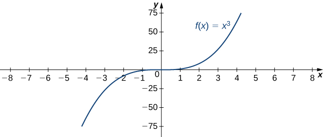
Figure $\PageIndex{8}$: For this function, the functional values approach $±$infinity as $x→±∞.$

Definition: infinite limit at infinity (Informal)

We say a function $f$ has an infinite limit at infinity and write

$$\lim_{x→∞}f(x)=∞.$$

if $f(x)$ becomes arbitrarily large for $x$ sufficiently large. We say a function has a negative infinite limit at infinity and write

$$\lim_{x→∞}f(x)=−∞.$$

if $f(x)<0$ and $|f(x)|$ becomes arbitrarily large for $x$ sufficiently large. Similarly, we can define infinite limits as $x→−∞.$

End Behavior

The behavior of a function as $x→±∞$ is called the function’s $end ;behavior$. At each of the function’s ends, the function could exhibit one of the following types of behavior:

1. The function $f(x)$ approaches a horizontal asymptote $y=L$.
2. The function $f(x)→∞$ or $f(x)→−∞.$
3. The function does not approach a finite limit, nor does it approach $∞$ or $−∞$. In this case, the function may have some oscillatory behavior.

Let’s consider several classes of functions here and look at the different types of end behaviors for these functions.

End Behavior for Polynomial Functions

Consider the power function $f(x)=x^n$ where $n$ is a positive integer. From Figure and Figure, we see that

$$\lim_{x→∞}x^n=∞;n=1,2,3,…$$

and

$$\lim_{x→−∞}x^n=\begin{cases}∞;n=2,4,6,…\\−∞;&n=1,3,5,….\end{cases}$$

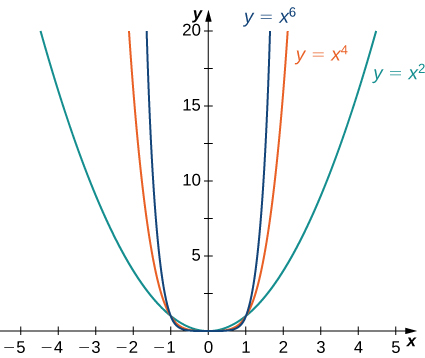
Figure $\PageIndex{11}$: For power functions with an even power of \(n, \displaystyle \lim_{x→∞}x^n=∞= \displaystyle \lim_{x→−∞}x^n\).

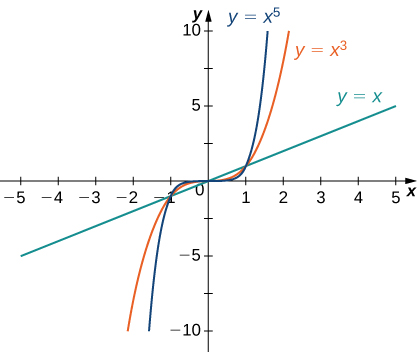
Figure $\PageIndex{12}$: For power functions with an odd power of \(n, \;\displaystyle \lim_{x→∞}x^n=∞\) and

$\displaystyle \lim_{x→−∞}x^n=−∞.$

Using these facts, it is not difficult to evaluate $\displaystyle \lim_{x→∞}cx^n$ and $\displaystyle \lim_{x→−∞}cx^n$, where $c$ is any constant and $n$ is a positive integer. If $c>0$, the graph of $y=cx^n$is a vertical stretch or compression of $y=x^n,$ and therefore

$\displaystyle \lim_{x→∞}cx^n=\lim_{x→∞}x^n$ and $\displaystyle \lim_{x→−∞}cx^n=\displaystyle \lim_{x→−∞}x^n$ if $c>0$.

If $c<0,$ the graph of $y=cx^n$ is a vertical stretch or compression combined with a reflection about the $x$-axis, and therefore

$\displaystyle \lim_{x→∞}cx^n=−\displaystyle \lim_{x→∞}x^n$ and $\displaystyle \lim_{x→−∞}cx^n=−\displaystyle \lim_{x→−∞}x^n$ if $c<0.$

If $c=0,y=cx^n=0,$ in which case $\displaystyle \lim_{x→∞}cx^n=0=\displaystyle \lim_{x→−∞}cx^n.$

Example $\PageIndex{4}$: Limits at Infinity for Power Functions

For each function $f$, evaluate $\displaystyle \lim_{x→∞}f(x)$ and $\displaystyle \lim_{x→−∞}f(x)$.

1. $f(x)=−5x^3$
2. $f(x)=2x^4$

Solution:

1. Since the coefficient of $x^3$ is $−5$, the graph of $f(x)=−5x^3$ involves a vertical stretch and reflection of the graph of $y=x^3$ about the $x$-axis. Therefore, $\displaystyle \lim_{x→∞}(−5x^3)=−∞$ and $\displaystyle \lim_{x→−∞}(−5x^3)=∞$.
2. Since the coefficient of $x^4$ is $2$, the graph of $f(x)=2x^4$ is a vertical stretch of the graph of $y=x^4$. Therefore, $\displaystyle \lim_{x→∞}2x^4=∞$ and $\displaystyle \lim_{x→−∞}2x^4=∞$.

Exercise $\PageIndex{4}$

Let $f(x)=−3x^4$. Find $\displaystyle \lim_{x→∞}f(x)$.

Hint

The coefficient $−3$ is negative.

Answer

$−∞$

We now look at how the limits at infinity for power functions can be used to determine $\displaystyle \lim_{x→±∞}f(x)$ for any polynomial function $f$. Consider a polynomial function

$$f(x)=a_nx^n+a_{n−1}x^{n−1}+…+a^1x+a^0$$

of degree $n≥1$ so that $a_n≠0.$Factoring, we see that

$$f(x)=a_nx^n(1+\frac{a_{n−1}}{a_n}\frac{1}{x}+…+\frac{a_1}{a_n}\frac{1}{x^{n−1}}+\frac{a_0}{a_n}\frac{1}{x^n}).$$

As $x→±∞,$ all the terms inside the parentheses approach zero except the first term. We conclude that

$$\lim_{x→±∞}f(x)=\lim_{x→±∞}a_nx^n.$$

For example, the function $f(x)=5x^3−3x^2+4$ behaves like $g(x)=5x^3$ as $x→±∞$ as shown in Figure and Table.

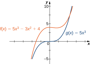
Figure $\PageIndex{13}$: The end behavior of a polynomial is determined by the behavior of the term with the largest exponent.

$x$	10	100	1000
$f(x)=5x^3−3x^2+4$	4704	4,970,004	4,997,000,004
$g(x)=5x^3$	5000	5,000,000	5,000,000,000
$x$	−10	−100	−000
$f(x)=5x^3−3x^2+4$	−5296	−5,029,996	−5,002,999,996
$g(x)=5x^3$	−5000	−5,000,000	−5,000,000,000

A polynomial’s end behavior is determined by the term with the largest exponent

End Behavior for Algebraic Functions

The end behavior for rational functions and functions involving radicals is a little more complicated than for polynomials. In Example, we show that the limits at infinity of a rational function $f(x)=\frac{p(x)}{q(x)}$ depend on the relationship between the degree of the numerator and the degree of the denominator. To evaluate the limits at infinity for a rational function, we divide the numerator and denominator by the highest power of $x$ appearing in the denominator. This determines which term in the overall expression dominates the behavior of the function at large values of $x$.

Example $\PageIndex{5}$: Determining End Behavior for Rational Functions

For each of the following functions, determine the limits as $x→∞$ and $x→−∞.$ Then, use this information to describe the end behavior of the function.

1. $f(x)=\frac{3x−1}{2x+5}$ (Note: The degree of the numerator and the denominator are the same.)
2. $f(x)=\frac{3x^2+2x}{4x^3−5x+7}$ (Note: The degree of numerator is less than the degree of the denominator.)
3. $f(x)=\frac{3x^2+4x}{x+2}$ in the denominator is x. Therefore, dividing the numerator and denominator by x and applying the algebraic limit laws, we see that

Solution

a. The highest power of $x$ in the denominator is $x$. Therefore, dividing the numerator and denominator by $x$ and applying the algebraic limit laws, we see that

$\displaystyle\lim_{x→±∞}\frac{3x−1}{2x+5}=\displaystyle \lim_{x→±∞}\frac{3−1/x}{2+5/x}$

$=\frac{\displaystyle \lim_{x→±∞}(3−1/x)}{\displaystyle \lim_{x→±∞}(2+5/x)}$

$=\frac{\displaystyle \lim_{x→±∞}3−\displaystyle \lim_{x→±∞}1/x}{\displaystyle \lim_{x→±∞}2+\displaystyle \lim_{x→±∞}5/x}$

$=\frac{3−0}{2+0}=\frac{3}{2}.$

Since $\displaystyle \lim_{x→±∞}f(x)=\frac{3}{2}$, we know that $y=\frac{3}{2}$ is a horizontal asymptote for this function as shown in the following graph.

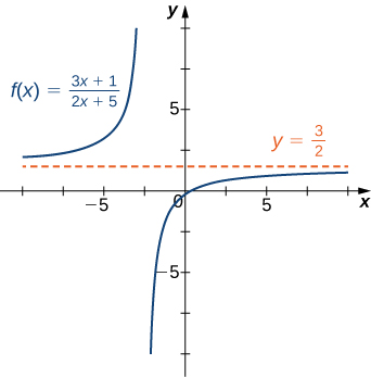
Figure $\PageIndex{14}$: The graph of this rational function approaches a horizontal asymptote as $x→±∞.$

b. Since the largest power of $x$ appearing in the denominator is $x^3$, divide the numerator and denominator by $x^3$. After doing so and applying algebraic limit laws, we obtain

$\displaystyle \lim_{x→±∞}\frac{3x^2+2x}{4x^3−5x+7}=\displaystyle \lim_{x→±∞}\frac{3/x+2/x^2}{4−5/x^2+7/x^3}=\frac{3.0+2.0}{4−5.0+7.0}=0.$

Therefore $f$ has a horizontal asymptote of $y=0$ as shown in the following graph.

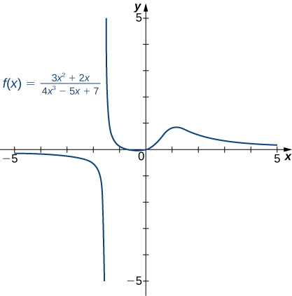
Figure $\PageIndex{15}$: The graph of this rational function approaches the horizontal asymptote \(y=0\) as $x→±∞.$

c. Dividing the numerator and denominator by $x$, we have

$\lim_{x→±∞}\frac{3x^2+4x}{x+2}=\lim_{x→±∞}\frac{3x+4}{1+2/x}$.

As $x→±∞$, the denominator approaches $1$. As $x→∞$, the numerator approaches $+∞$. As $x→−∞$, the numerator approaches $−∞$. Therefore $\lim_{x→∞}f(x)=∞$, whereas $\lim_{x→−∞}f(x)=−∞$ as shown in the following figure.

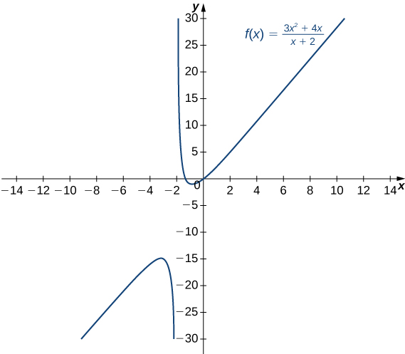
Figure $\PageIndex{16}$: As $→∞$, the values $f(x)→∞$. As $x→−∞$, the values $f(x)→−∞.$

Exercise $\PageIndex{5}$

Evaluate $\displaystyle \lim_{x→±∞}\frac{3x^2+2x−1}{5x^2−4x+7}$ and use these limits to determine the end behavior of $f(x)=\frac{3x^2+2x−2}{5x^2−4x+7}$.

Hint

Divide the numerator and denominator by $x^2$.

Answer

$\frac{3}{5}$

Before proceeding, consider the graph of $f(x)=\frac{(3x^2+4x)}{(x+2)}$ shown in Figure. As $x→∞$ and $x→−∞$, the graph of $f$ appears almost linear. Although $f$ is certainly not a linear function, we now investigate why the graph of $f$ seems to be approaching a linear function. First, using long division of polynomials, we can write

$f(x)=\frac{3x^2+4x}{x+2}=3x−2+\frac{4}{x+2}$.

Since $\frac{4}{(x+2)}→0$ as $x→±∞,$ we conclude that

$\displaystyle \lim_{x→±∞}(f(x)−(3x−2))=\displaystyle \lim_{x→±∞}\frac{4}{x+2}=0.$

Therefore, the graph of $f$ approaches the line \)y=3x−2\) as $x→±∞$. This line is known as an oblique asymptote for $f$ (Figure).

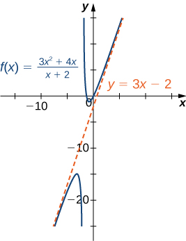
Figure $\PageIndex{17}$: The graph of the rational function $f(x)=(3x^2+4x)/(x+2)$ approaches the oblique asymptote $y=3x−2$ as $x→±∞.$

We can summarize the results of Example to make the following conclusion regarding end behavior for rational functions. Consider a rational function

$f(x)=\frac{p(x)}{q(x)}=\frac{a_nx^n+a_{n−1}x^{n−1}+…+a_1x+a_0}{b_mx^m+b_{m−1}x^{m−1}+…+b_1x+b_0}$,

where $a_n≠0$ and $b_m≠0.$

1. If the degree of the numerator is the same as the degree of the denominator $(n=m),$ then $f$ has a horizontal asymptote of $y=a_n/b_m$ as $x→±∞.$

2. If the degree of the numerator is less than the degree of the denominator $(n<m),$ then $f$ has a horizontal asymptote of $y=0$ as $x→±∞.$

3. If the degree of the numerator is greater than the degree of the denominator $(n>m),$ then $f$ does not have a horizontal asymptote. The limits at infinity are either positive or negative infinity, depending on the signs of the leading terms. In addition, using long division, the function can be rewritten as

$f(x)=\frac{p(x)}{q(x)}=g(x)+\frac{r(x)}{q(x)}$,

where the degree of $r(x)$ is less than the degree of $q(x)$. As a result, $\displaystyle \lim_{x→±∞}r(x)/q(x)=0$. Therefore, the values of $[f(x)−g(x)]$ approach zero as $x→±∞$. If the degree of $p(x)$ is exactly one more than the degree of $q(x) (n=m+1)$, the function $g(x)$ is a linear function. In this case, we call $g(x)$ an oblique asymptote.

Now let’s consider the end behavior for functions involving a radical.

Example $\PageIndex{6}$: Determining End Behavior for a Function Involving a Radical

Find the limits as $x→∞$ and $x→−∞$ for $f(x)=\frac{3x−2}{\sqrt{4x^2+5}}$ and describe the end behavior of $f$.

Solution

Let’s use the same strategy as we did for rational functions: divide the numerator and denominator by a power of $x$. To determine the appropriate power of $x$, consider the expression $\sqrt{4x^2+5}$ in the denominator. Since

$$\sqrt{4x^2+5}≈\sqrt{4x^2}=2|x|$$

for large values of $x$ in effect $x$ appears just to the first power in the denominator. Therefore, we divide the numerator and denominator by $|x|$. Then, using the fact that $|x|=x$ for $x>0, |x|=−x$ for $x<0$, and $|x|=\sqrt{x^2}$ for all $x$, we calculate the limits as follows:

$\displaystyle\lim_{x→∞}\frac{3x−2}{\sqrt{4x^2+5}}=\displaystyle\lim_{x→∞}\frac{(1/|x|)(3x−2)}{(1/|x|)\sqrt{4x^2+5}}$

$=\displaystyle\lim_{x→∞}\frac{(1/x)(3x−2)}{\sqrt{(1/x^2)(4x^2+5)}}$

$=\displaystyle\lim_{x→∞}\frac{3−2/x}{\sqrt{4+5/x^2}}=\frac{3}{\sqrt{4}}=\frac{3}{2}$

$\displaystyle\lim_{x→−∞}\frac{3x−2}{\sqrt{4x^2+5}}=\lim_{x→−∞}\frac{(1/|x|)(3x−2)}{(1/|x|)\sqrt{4x^2+5}}$

$=\displaystyle\lim_{x→−∞}\frac{(−1/x)(3x−2)}{\sqrt{(1/x^2)(4x^2+5)}}$

$=\displaystyle\lim_{x→−∞}\frac{−3+2/x}{\sqrt{4+5/x^2}}=\frac{−3}{\sqrt{4}}=\frac{−3}{2}$.

Therefore, $f(x)$ approaches the horizontal asymptote $y=\frac{3}{2}$ as $x→∞$ and the horizontal asymptote $y=−\frac{3}{2}$ as $x→−∞$ as shown in the following graph.

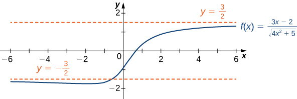
Figure $\PageIndex{18}$:This function has two horizontal asymptotes and it crosses one of the asymptotes.

Exercise $\PageIndex{6}$

Evaluate $\displaystyle\lim_{x→∞}\frac{\sqrt{3x^2+4}}{x+6}$.

Hint

Divide the numerator and denominator by $|x|.$

Answer

$\sqrt{3}$

Determining End Behavior for Transcendental Functions

The six basic trigonometric functions are periodic and do not approach a finite limit as $x→±∞.$ For example, $sinx$ oscillates between $1and−1$ (Figure). The tangent function $x$ has an infinite number of vertical asymptotes as $x→±∞$; therefore, it does not approach a finite limit nor does it approach $±∞$ as $x→±∞$ as shown in Figure.

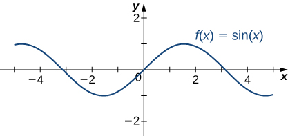
Figure $\PageIndex{19}$:The function $f(x)=sinx$ oscillates between $1and−1$ as $x→±∞$

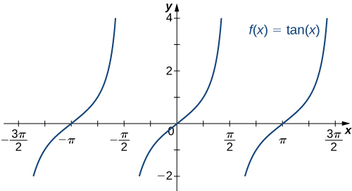
Figure $\PageIndex{20}$: The function $f(x)=tanx$ does not approach a limit and does not approach $±∞$ as $x→±∞$

Recall that for any base $b>0,b≠1,$ the function $y=b^x$ is an exponential function with domain $(−∞,∞)$ and range $(0,∞)$. If $b>1,y=b^x$ is increasing over `$(−∞,∞)$. If $0<b<1, y=b^x$ is decreasing over $(−∞,∞).$ For the natural exponential function $f(x)=e^x, e≈2.718>1$. Therefore, $f(x)=e^x$ is increasing on `$(−∞,∞)$ and the range is `$(0,∞).$ The exponential function $f(x)=e^x$ approaches $∞$ as $x→∞$ and approaches $0$ as $x→−∞$ as shown in Table and Figure.

End behavior of the natural exponential function

$x$	−5	−2	0	2	5
$e^x$	0.00674	0.135	1	7.389	148.413

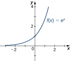
Figure $\PageIndex{21}$: The exponential function approaches zero as $x→−∞$ and approaches $∞$ as $x→∞.$

Recall that the natural logarithm function $f(x)=ln(x)$ is the inverse of the natural exponential function $y=e^x$. Therefore, the domain of $f(x)=ln(x)$ is $(0,∞)$ and the range is $(−∞,∞)$. The graph of $f(x)=ln(x)$ is the reflection of the graph of $y=e^x$ about the line $y=x$. Therefore, $ln(x)→−∞$ as $x→0^+$ and $ln(x)→∞$ as $x→∞$ as shown in Figure and Table.

End behavior of the natural logarithm function

$x$	0.01	0.1	1	10	100
$ln(x)$	−4.605	−2.303	0	2.303	4.605

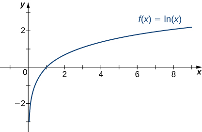
Figure $\PageIndex{22}$: The natural logarithm function approaches $∞$ as $x→∞.$

Example $\PageIndex{7}$: Determining End Behavior for a Transcendental Function

Find the limits as $x→∞$ and $x→−∞$ for $f(x)=\frac{(2+3e^x)}{(7−5e^x)}$ and describe the end behavior of $f.$

Solution

To find the limit as $x→∞,$ divide the numerator and denominator by $e^x$:

$\displaystyle\lim_{x→∞}f(x)=\displaystyle \lim_{x→∞}\frac{2+3e^x}{7−5e^x}$

$=\displaystyle \lim_{x→∞}\frac{(2/e^x)+3}{(7/e^x)−5.}$

As shown in Figure, $e^x→∞$ as $x→∞.$ Therefore,

$\displaystyle \lim_{x→∞}\frac{2}{e^x}=0=\displaystyle \lim_{x→∞}\frac{7}{e^x}$.

We conclude that $\displaystyle \lim_{x→∞f}(x)=−\frac{3}{5}$, and the graph of $f$ approaches the horizontal asymptote $y=−\frac{3}{5}$ as $x→∞.$ To find the limit as $x→−∞$, use the fact that $e^x→0$ as $x→−∞$ to conclude that $\displaystyle \lim_{x→∞}f(x)=\frac{2}{7}$, and therefore the graph of approaches the horizontal asymptote $y=\frac{2}{7}$ as $x→−∞$.

Exercise $\PageIndex{7}$

Find the limits as $x→∞$ and $x→−∞$ for $f(x)=\frac{(3e^x−4)}{(5e^x+2).}$

Hint

$\displaystyle\lim_{x→∞}e^x=∞$ and $\displaystyle \lim_{x→∞}e^x=0.$

Answer

$\displaystyle\lim_{x→∞}f(x)=\frac{3}{5}, \displaystyle \lim_{x→−∞}f(x)=−2$

Key Concepts

• The limit of $f(x)$ is $L$ as $x→∞$ (or as $x→−∞)$ if the values $f(x)$ become arbitrarily close to $L$ as $x$becomes sufficiently large.
• The limit of $f(x)$ is $∞$ as $x→∞$ if $f(x)$ becomes arbitrarily large as $x$ becomes sufficiently large. The limit of $f(x)$ is $−∞$ as $x→∞$ if $f(x)<0$ and $|f(x)|$ becomes arbitrarily large as $x$ becomes sufficiently large. We can define the limit of $f(x)$ as $x$ approaches $−∞$ similarly.
• For a polynomial function $p(x)=a_nx^n+a_{n−1}x^{n−1}+…+a_1x+a_0,$ where $a_n≠0$, the end behavior is determined by the leading term $a_nx^n$. If $n≠0, p(x)$ approaches $∞$ or $−∞$at each end.
• For a rational function $f(x)=\frac{p(x)}{q(x),}$ the end behavior is determined by the relationship between the degree of $p$ and the degree of $q$. If the degree of $p$ is less than the degree of $q$, the line $y=0$ is a horizontal asymptote for $f$. If the degree of $p$ is equal to the degree of $q$, then the line $y=\frac{a_n}{b_n}$ is a horizontal asymptote, where $a_n$ and $b_n$ are the leading coefficients of $p$ and $q$, respectively. If the degree of $p$ is greater than the degree of $q$, then $f$ approaches $∞$ or $−∞$ at each end. NOTE: These rules are good to check your work, but be aware that you need to justify your conclusions with Calculus, namely working out the limits as $x$ approaches $∞$ or $−∞$.

Glossary

end behavior

the behavior of a function as $x→∞$ and $x→−∞$

horizontal asymptote

if \displaystyle(\lim_{x→∞}f(x)=L\) or $\displaystyle\lim_{x→−∞}f(x)=L$, then $y=L$ is a horizontal asymptote of $f$

infinite limit at infinity

a function that becomes arbitrarily large as x becomes large

limit at infinity

a function that becomes arbitrarily large as $x$ becomes large

oblique asymptote

the line $y=mx+b$ if $f(x)$ approaches it as $x→∞$ or $x→−∞$

Contributors

• Gilbert Strang (MIT) and Edwin “Jed” Herman (Harvey Mudd) with many contributing authors. This content by OpenStax is licensed with a CC-BY-SA-NC 4.0 license. Download for free at http://cnx.org.