4.4 E: Sketch the GRAPH Exercises

4.4: Graphing Exercises

For the following exercises, draw a graph of the functions without using a calculator. Use the 9-step process for graphing from Class Notes and from the section 4.5 text.

The answers here are just the graph (step 9). Your solutions should have all steps with the information (intervals of incr/decr, local max/min, etc) as you see in the section 4.5 text examples.

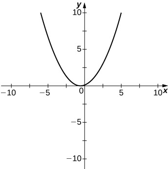
294) \(y=3x^2+2x+4\)

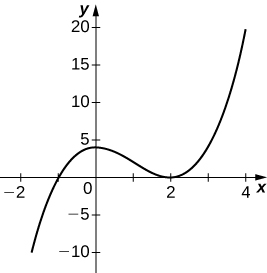
295) \(y=x^3−3x^2+4\)

Answer:

Note: should have a hole at the point (-3,2)

296) \(y=\frac{2x+1}{x^2+6x+5}\)

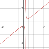
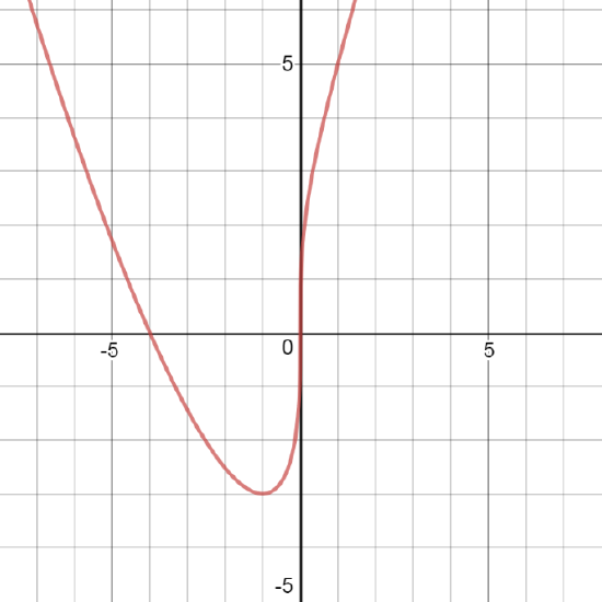
297) \(y=\frac{x^3+4x^2+3x}{3x+9}\)

Answer:

298) \(y=\frac{x^2+x−2}{x^2−3x−4}\)

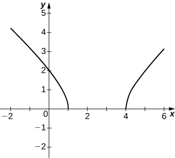
299) \(y=\sqrt{x^2−5x+4}\)

Answer:

300) \(y=2x\sqrt{16−x^2}\)

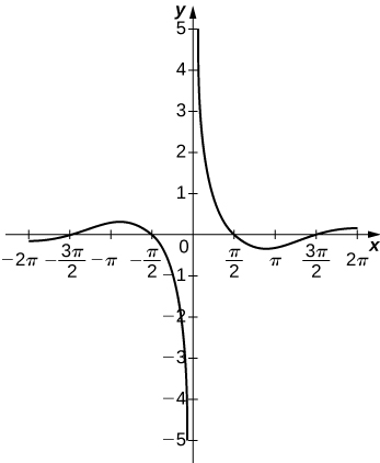
301) \(y=\frac{cosx}{x}\), on \(x=[−2π,2π]\)

Answer:

302) \(y=e^x−x^3\)

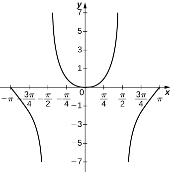
303) \(y=x \tan x,x=[−π,π]\)

Answer:

304) \(y=x\ln(x),x>0\)

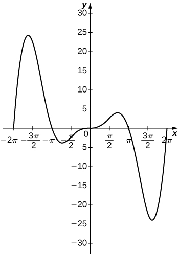
305) \(y=x^2\sin(x),x=[−2π,2π]\)

Answer:

306) For \(f(x)=\frac{P(x)}{Q(x)}\) to have an asymptote at \(y=2\) then the polynomials \(P(x)\) and \(Q(x)\) must have what relation?

307) For \(f(x)=\frac{P(x)}{Q(x)}\) to have an asymptote at \(x=0\), then the polynomials \(P(x)\) and \(Q(x).\) must have what relation?

Answer:

\(Q(x).\) must have have \(x^{k+1}\) as a factor, where \(P(x)\) has \(x^k\) as a factor.

308) If \(f′(x)\) has asymptotes at \(y=3\) and \(x=1\), then \(f(x)\) has what asymptotes?

309) Both \(f(x)=\frac{1}{(x−1)}\) and \(g(x)=\frac{1}{(x−1)^2}\) have asymptotes at \(x=1\) and \(y=0.\) What is the most obvious difference between these two functions?

Answer:

\(\displaystyle lim_{x→1^−f(x)and \displaystyle lim_x→1−g(x)

310) True or false: Every ratio of polynomials has vertical asymptotes.

---

For the following exercises, draw a graph of the functions without using a calculator. Use the 9-step process for graphing from Class Notes and from the section 4.4 text. Your solutions should have all steps with the information (intervals of incr/decr, local max/min, etc) as you see in the section 4.4 text examples.

J4.4.1) \(y=\frac{x^2+2}{x^2-4}\)

J4.4.2) \(f(x)=x-3x^{\frac{1}{3}}\)

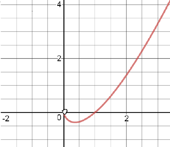
J4.4.3) \(f(x)=x\ln x\)

Answer:

Domain (0, ∞); Intercept (0,1); Symmetry Not odd, Not even; VA none, HA none, as x → ∞ , f → ∞;
increasing on \((\frac{1}{e}, ∞)\); decreasing on \((0, \frac{1}{e})\); min \((\frac{1}{e}, -\frac{1}{e})\); no max;
concave up (0, ∞); never concave down; no inflection point

J4.4.4) \(f(x)=x^4-6x^2\)

J4.4.5) \(f(x)=\frac{x^2}{x-2}\)

Answer:

Domain \(x≠2\) ; Intercept (0,0); Symmetry Not odd, Not even; VA \(x=2\), HA none, as \(x → ∞\) , \(f → ∞\); as \(x →- ∞\) , \(f → -∞\);
increasing on \( (-∞,0)\) \((4, ∞,)\), decreasing on \((0, 2)\) \((2,4)\); min \((4,8)\); max;\((0,0)\);
concave up (2, ∞), concave down (-∞ , 2); inflection points \((-\sqrt{2},\frac{2}{-\sqrt{2}-2})\), \((\sqrt{2},\frac{2}{\sqrt{2}-2})\)

J4.4.6) \(f(x)=\frac{x^2-2}{x^4}\)

J4.4.7) \(f(x)=4x^{\frac{1}{3}}+x^{\frac{4}{3}}\)

Answer:

Domain (-∞, ∞); Intercepts (-4,0) (0,0); Symmetry Not odd, Not even; VA none, HA none, as \( x→±∞ \) , \(f → ∞\);
increasing on \( (-1,∞)\); decreasing on \((-∞,-1,)\); min \((-1,-3)\); max none;
concave up \( (-∞,0)\) \((2, ∞,)\); concave down (0, 2); inflection points \((2,6\sqrt[3]{2})\)

J4.4.8) \(f(x)=\frac{1}{(1+e^x)^2}\)

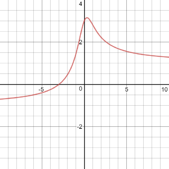
J4.4.9) \(f(x)=\frac{x+3}{\sqrt{x^2+1}}\)

Answer:

Domain (-∞, ∞); Intercepts (-3,0), (0,3); Symmetry Not odd, Not even; VA none, HA \(y=-1\) (as \(x→-∞ \)) , HA \(y=1\) (as \(x→∞\));
increasing on \((-∞,\frac{1}{3})\); decreasing on \( (\frac{1}{3},∞)\); max \((\frac{1}{3},\sqrt{10})\); min none;
concave up \( (-∞,-\frac{1}{2})\), \((1,∞)\);concave down \( (-\frac{1}{2},1)\); inflection points \( (-\frac{1}{2},\sqrt{5})\), \((1,2\sqrt{2})\)