
5.1: Approximating Areas


- Last updated
- Dec 21, 2020
- Save as PDF

( \newcommand{\kernel}{\mathrm{null}\,}\)
Archimedes was fascinated with calculating the areas of various shapes—in other words, the amount of space enclosed by the shape. He used a process that has come to be known as the method of exhaustion, which used smaller and smaller shapes, the areas of which could be calculated exactly, to fill an irregular region and thereby obtain closer and closer approximations to the total area. In this process, an area bounded by curves is filled with rectangles, triangles, and shapes with exact area formulas. These areas are then summed to approximate the area of the curved region.
In this section, we develop techniques to approximate the area between a curve, defined by a function
Let’s start by introducing some notation to make the calculations easier. We then consider the case when
Sigma (Summation) Notation
As mentioned, we will use shapes of known area to approximate the area of an irregular region bounded by curves. This process often requires adding up long strings of numbers. To make it easier to write down these lengthy sums, we look at some new notation here, called sigma notation (also known as summation notation). The Greek capital letter
We could probably skip writing a couple of terms and write
which is better, but still cumbersome. With sigma notation, we write this sum as
which is much more compact. Typically, sigma notation is presented in the form
where
is interpreted as
Note that the index is used only to keep track of the terms to be added; it does not factor into the calculation of the sum itself. The index is therefore called a dummy variable. We can use any letter we like for the index. Typically, mathematicians use
Let’s try a couple of examples of using sigma notation.
Example
- Write in sigma notation and evaluate the sum of terms
- Write the sum in sigma notation:
Solution
- Write
- The denominator of each term is a perfect square. Using sigma notation, this sum can be written as
Exercise
Write in sigma notation and evaluate the sum of terms
- Hint
-
Use the solving steps in Example
- Answer
-
The properties associated with the summation process are given in the following rule.
Rule: Properties of Sigma Notation
Let
Proof
We prove properties 2. and 3. here, and leave proof of the other properties to the exercises below.
2. We have
3. We have
□
A few more formulas for frequently found functions simplify the summation process further. These are shown in the next rule, for sums and powers of integers, and we use them in the next set of examples.
Rule: Sums and Powers of Integers
1. The sum of n integers is given by
2. The sum of consecutive integers squared is given by
3. The sum of consecutive integers cubed is given by
Example
Write using sigma notation and evaluate:
- The sum of the terms
- The sum of the terms
Solution
a. Multiplying out
b. Use sigma notation property iv. and the rules for the sum of squared terms and the sum of cubed terms.
Exercise
Find the sum of the values of
- Hint
-
Use the properties of sigma notation to solve the problem.
- Answer
-
15,550
Example
Find the sum of the values of
Solution
Using the the rule for sum of consecutive integers cubed (Equation
Exercise
Evaluate the sum indicated by the notation
- Hint
-
Use the rule on sum and powers of integers.
- Answer
-
440
Approximating Area
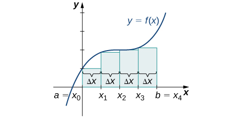
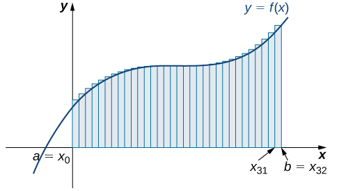
Now that we have the necessary notation, we return to the problem at hand: approximating the area under a curve. Let
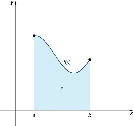
Figure
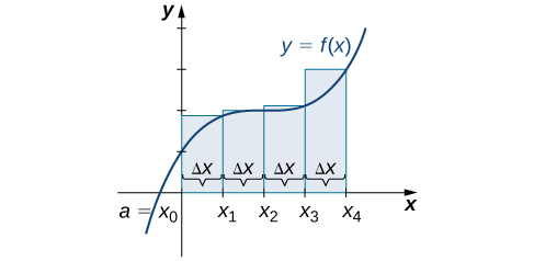
How do we approximate the area under this curve? The approach is a geometric one. By dividing a region into many small shapes that have known area formulas, we can sum these areas and obtain a reasonable estimate of the true area. We begin by dividing the interval
for
We denote the width of each subinterval with the notation Δx, so
for
Definition: Partitions
A set of points
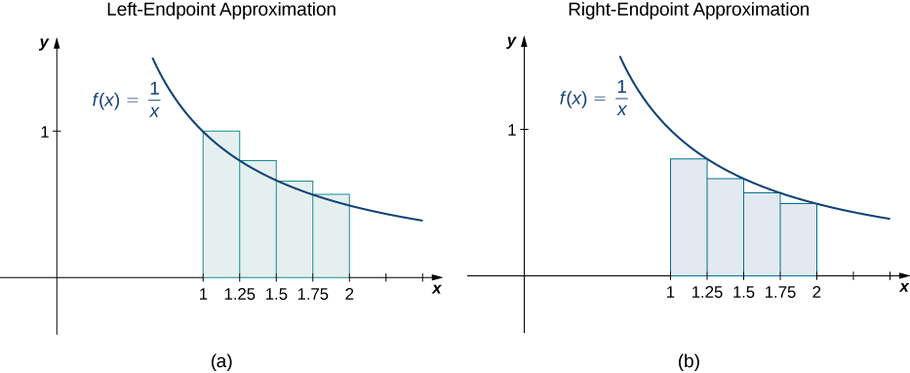
We can use this regular partition as the basis of a method for estimating the area under the curve. We next examine two methods: the left-endpoint approximation and the right-endpoint approximation.
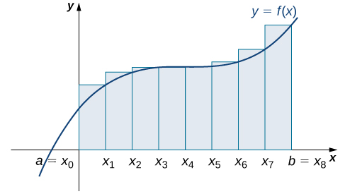
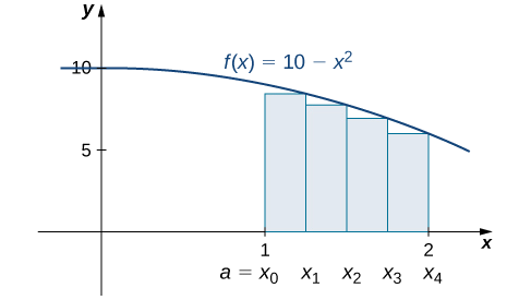
Rule: Left-Endpoint Approximation
On each subinterval
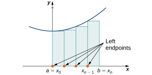
Figure
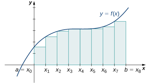
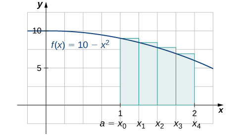
The second method for approximating area under a curve is the right-endpoint approximation. It is almost the same as the left-endpoint approximation, but now the heights of the rectangles are determined by the function values at the right of each subinterval.
Rule: Right-Endpoint Approximation
Construct a rectangle on each subinterval
The notation
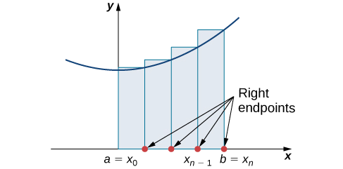
Figure
The graphs in Figure
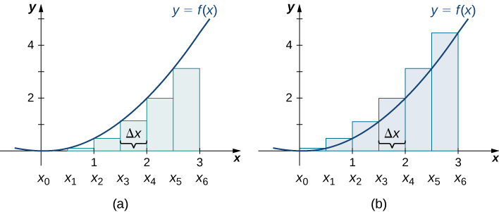
Figure
In Figure
In Figure
Example
Use both left-endpoint and right-endpoint approximations to approximate the area under the curve of
Solution
First, divide the interval
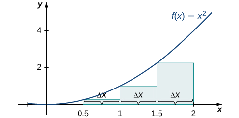
Figure
The right-endpoint approximation is shown in Figure
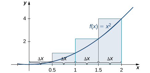
Figure
The left-endpoint approximation is 1.75; the right-endpoint approximation is 3.75.
Exercise
Sketch left-endpoint and right-endpoint approximations for
- Hint
-
Follow the solving strategy in Example
- Answer
-
The left-endpoint approximation (Equation
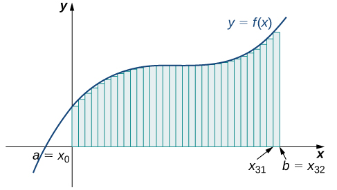
Looking at Figure
We can demonstrate the improved approximation obtained through smaller intervals with an example. Let’s explore the idea of increasing
The area is approximated by the summed areas of the rectangles, or
Figure
Figure
Figure
The graph in Figure
Figure
We can carry out a similar process for the right-endpoint approximation method. A right-endpoint approximation of the same curve, using four rectangles (Figure
Figure
Dividing the region over the interval
Figure
Last, the right-endpoint approximation with
Figure
Based on these figures and calculations, it appears we are on the right track; the rectangles appear to approximate the area under the curve better as n gets larger. Furthermore, as n increases, both the left-endpoint and right-endpoint approximations appear to approach an area of 8 square units. Table shows a numerical comparison of the left- and right-endpoint methods. The idea that the approximations of the area under the curve get better and better as n gets larger and larger is very important, and we now explore this idea in more detail.
| Value of n | Approximate Area |
Approximate Area |
|---|---|---|
| 7.5 | 8.5 | |
| 7.75 | 8.25 | |
| 7.94 | 8.06 |
Forming Riemann Sums
So far we have been using rectangles to approximate the area under a curve. The heights of these rectangles have been determined by evaluating the function at either the right or left endpoints of the subinterval
A sum of this form is called a Riemann sum, named for the 19th-century mathematician Bernhard Riemann, who developed the idea.
Note
Let
Recall that with the left- and right-endpoint approximations (Equations
We look at some examples shortly. But, before we do, let’s take a moment and talk about some specific choices for
If we want an overestimate, for example, we can choose
Example
Find a lower sum for
Solution
With
Figure
The Riemann sum is
The area of 7.28 is a lower sum and an underestimate.
Exercise
- Find an upper sum for
- Sketch the approximation.
- Hint
-
- Answer
-
a. Upper sum=
b.
Example
Find a lower sum for
Solution
Let’s first look at the graph in Figure to get a better idea of the area of interest.
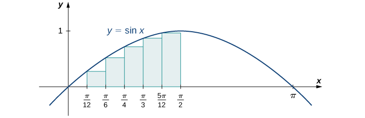
Figure
The intervals are
Exercise
Using the function
- Hint
-
Follow the steps from Example
- Answer
-
Key Concepts
- The use of sigma (summation) notation of the form
- For a continuous function defined over an interval
- The width of each rectangle is
- Riemann sums are expressions of the form
- Riemann sums allow for much flexibility in choosing the set of points
Key Equations
- Properties of Sigma Notation
- Sums and Powers of Integers
- Left-Endpoint Approximation
- Right-Endpoint Approximation
Glossary
- left-endpoint approximation
- an approximation of the area under a curve computed by using the left endpoint of each subinterval to calculate the height of the vertical sides of each rectangle
- lower sum
- a sum obtained by using the minimum value of \(f(x)\) on each subinterval
- partition
- a set of points that divides an interval into subintervals
- regular partition
- a partition in which the subintervals all have the same width
- riemann sum
- an estimate of the area under the curve of the form
- right-endpoint approximation
- the right-endpoint approximation is an approximation of the area of the rectangles under a curve using the right endpoint of each subinterval to construct the vertical sides of each rectangle
- sigma notation
- (also, summation notation) the Greek letter sigma (
- upper sum
- a sum obtained by using the maximum value of \(f(x)\) on each subinterval
Contributors
Gilbert Strang (MIT) and Edwin “Jed” Herman (Harvey Mudd) with many contributing authors. This content by OpenStax is licensed with a CC-BY-SA-NC 4.0 license. Download for free at http://cnx.org.