5.4: Average Value of a Function

Last updated
Save as PDF

Page ID: 13816

$ \newcommand{\vecs}[1]{\overset { \scriptstyle \rightharpoonup} {\mathbf{#1}} } $

$ \newcommand{\vecd}[1]{\overset{-\!-\!\rightharpoonup}{\vphantom{a}\smash {#1}}} $

$ \newcommand{\id}{\mathrm{id}}$ $ \newcommand{\Span}{\mathrm{span}}$

( \newcommand{\kernel}{\mathrm{null}\,}\) $ \newcommand{\range}{\mathrm{range}\,}$

$ \newcommand{\RealPart}{\mathrm{Re}}$ $ \newcommand{\ImaginaryPart}{\mathrm{Im}}$

$ \newcommand{\Argument}{\mathrm{Arg}}$ $ \newcommand{\norm}[1]{\| #1 \|}$

$ \newcommand{\inner}[2]{\langle #1, #2 \rangle}$

$ \newcommand{\Span}{\mathrm{span}}$

$ \newcommand{\id}{\mathrm{id}}$

$ \newcommand{\Span}{\mathrm{span}}$

$ \newcommand{\kernel}{\mathrm{null}\,}$

$ \newcommand{\range}{\mathrm{range}\,}$

$ \newcommand{\RealPart}{\mathrm{Re}}$

$ \newcommand{\ImaginaryPart}{\mathrm{Im}}$

$ \newcommand{\Argument}{\mathrm{Arg}}$

$ \newcommand{\norm}[1]{\| #1 \|}$

$ \newcommand{\inner}[2]{\langle #1, #2 \rangle}$

$ \newcommand{\Span}{\mathrm{span}}$ $ \newcommand{\AA}{\unicode[.8,0]{x212B}}$

$ \newcommand{\vectorA}[1]{\vec{#1}} % arrow$

$ \newcommand{\vectorAt}[1]{\vec{\text{#1}}} % arrow$

$ \newcommand{\vectorB}[1]{\overset { \scriptstyle \rightharpoonup} {\mathbf{#1}} } $

$ \newcommand{\vectorC}[1]{\textbf{#1}} $

$ \newcommand{\vectorD}[1]{\overrightarrow{#1}} $

$ \newcommand{\vectorDt}[1]{\overrightarrow{\text{#1}}} $

$ \newcommand{\vectE}[1]{\overset{-\!-\!\rightharpoonup}{\vphantom{a}\smash{\mathbf {#1}}}} $

$ \newcommand{\vecs}[1]{\overset { \scriptstyle \rightharpoonup} {\mathbf{#1}} } $

$ \newcommand{\vecd}[1]{\overset{-\!-\!\rightharpoonup}{\vphantom{a}\smash {#1}}} $

$\newcommand{\avec}{\mathbf a}$ $\newcommand{\bvec}{\mathbf b}$ $\newcommand{\cvec}{\mathbf c}$ $\newcommand{\dvec}{\mathbf d}$ $\newcommand{\dtil}{\widetilde{\mathbf d}}$ $\newcommand{\evec}{\mathbf e}$ $\newcommand{\fvec}{\mathbf f}$ $\newcommand{\nvec}{\mathbf n}$ $\newcommand{\pvec}{\mathbf p}$ $\newcommand{\qvec}{\mathbf q}$ $\newcommand{\svec}{\mathbf s}$ $\newcommand{\tvec}{\mathbf t}$ $\newcommand{\uvec}{\mathbf u}$ $\newcommand{\vvec}{\mathbf v}$ $\newcommand{\wvec}{\mathbf w}$ $\newcommand{\xvec}{\mathbf x}$ $\newcommand{\yvec}{\mathbf y}$ $\newcommand{\zvec}{\mathbf z}$ $\newcommand{\rvec}{\mathbf r}$ $\newcommand{\mvec}{\mathbf m}$ $\newcommand{\zerovec}{\mathbf 0}$ $\newcommand{\onevec}{\mathbf 1}$ $\newcommand{\real}{\mathbb R}$ $\newcommand{\twovec}[2]{\left[\begin{array}{r}#1 \\ #2 \end{array}\right]}$ $\newcommand{\ctwovec}[2]{\left[\begin{array}{c}#1 \\ #2 \end{array}\right]}$ $\newcommand{\threevec}[3]{\left[\begin{array}{r}#1 \\ #2 \\ #3 \end{array}\right]}$ $\newcommand{\cthreevec}[3]{\left[\begin{array}{c}#1 \\ #2 \\ #3 \end{array}\right]}$ $\newcommand{\fourvec}[4]{\left[\begin{array}{r}#1 \\ #2 \\ #3 \\ #4 \end{array}\right]}$ $\newcommand{\cfourvec}[4]{\left[\begin{array}{c}#1 \\ #2 \\ #3 \\ #4 \end{array}\right]}$ $\newcommand{\fivevec}[5]{\left[\begin{array}{r}#1 \\ #2 \\ #3 \\ #4 \\ #5 \\ \end{array}\right]}$ $\newcommand{\cfivevec}[5]{\left[\begin{array}{c}#1 \\ #2 \\ #3 \\ #4 \\ #5 \\ \end{array}\right]}$ $\newcommand{\mattwo}[4]{\left[\begin{array}{rr}#1 \amp #2 \\ #3 \amp #4 \\ \end{array}\right]}$ $\newcommand{\laspan}[1]{\text{Span}\{#1\}}$ $\newcommand{\bcal}{\cal B}$ $\newcommand{\ccal}{\cal C}$ $\newcommand{\scal}{\cal S}$ $\newcommand{\wcal}{\cal W}$ $\newcommand{\ecal}{\cal E}$ $\newcommand{\coords}[2]{\left\{#1\right\}_{#2}}$ $\newcommand{\gray}[1]{\color{gray}{#1}}$ $\newcommand{\lgray}[1]{\color{lightgray}{#1}}$ $\newcommand{\rank}{\operatorname{rank}}$ $\newcommand{\row}{\text{Row}}$ $\newcommand{\col}{\text{Col}}$ $\renewcommand{\row}{\text{Row}}$ $\newcommand{\nul}{\text{Nul}}$ $\newcommand{\var}{\text{Var}}$ $\newcommand{\corr}{\text{corr}}$ $\newcommand{\len}[1]{\left|#1\right|}$ $\newcommand{\bbar}{\overline{\bvec}}$ $\newcommand{\bhat}{\widehat{\bvec}}$ $\newcommand{\bperp}{\bvec^\perp}$ $\newcommand{\xhat}{\widehat{\xvec}}$ $\newcommand{\vhat}{\widehat{\vvec}}$ $\newcommand{\uhat}{\widehat{\uvec}}$ $\newcommand{\what}{\widehat{\wvec}}$ $\newcommand{\Sighat}{\widehat{\Sigma}}$ $\newcommand{\lt}{<}$ $\newcommand{\gt}{>}$ $\newcommand{\amp}{&}$ $\definecolor{fillinmathshade}{gray}{0.9}$

5.4 Average Value of a Function

We often need to find the average of a set of numbers, such as an average test grade. Suppose you received the following test scores in your algebra class: 89, 90, 56, 78, 100, and 69. Your semester grade is your average of test scores and you want to know what grade to expect. We can find the average by adding all the scores and dividing by the number of scores. In this case, there are six test scores. Thus,

\[\dfrac{89+90+56+78+100+69}{6}=\dfrac{482}{6}≈80.33.\]

Therefore, your average test grade is approximately 80.33, which translates to a B− at most schools.

Suppose, however, that we have a function $v(t)$ that gives us the speed of an object at any time t, and we want to find the object’s average speed. The function $v(t)$ takes on an infinite number of values, so we can’t use the process just described. Fortunately, we can use a definite integral to find the average value of a function such as this.

Let $f(x)$ be continuous over the interval $[a,b]$ and let $[a,b]$ be divided into n subintervals of width $Δx=(b−a)/n$. Choose a representative $x^∗_i$ in each subinterval and calculate $f(x^∗_i)$ for $i=1,2,…,n.$ In other words, consider each $f(x^∗_i)$ as a sampling of the function over each subinterval. The average value of the function may then be approximated as

\[\dfrac{f(x^∗_1)+f(x^∗_2)+⋯+f(x^∗_n)}{n},\]

which is basically the same expression used to calculate the average of discrete values.

But we know $Δx=\dfrac{b−a}{n},$ so $n=\dfrac{b−a}{Δx}$, and we get

\[\dfrac{f(x^∗_1)+f(x^∗_2)+⋯+f(x^∗_n)}{n}=\dfrac{f(x^∗_1)+f(x^∗_2)+⋯+f(x^∗_n)}{\dfrac{(b−a)}{Δx}}.\]

Following through with the algebra, the numerator is a sum that is represented as $\sum_{i=1}^nf(x∗i),$ and we are dividing by a fraction. To divide by a fraction, invert the denominator and multiply. Thus, an approximate value for the average value of the function is given by

$\dfrac{\sum_{i=1}^nf(x^∗_i)}{\dfrac{(b−a)}{Δx}}=(\dfrac{Δx}{b−a})\sum_{i=1}^nf(x^∗_i)=(\dfrac{1}{b−a})\sum_{i=1}^nf(x^∗_i)Δx.$

This is a Riemann sum. Then, to get the exact average value, take the limit as n goes to infinity. Thus, the average value of a function is given by

$\dfrac{1}{b−a}\lim_{n→∞}\sum_{i=1}^nf(x_i)Δx=\dfrac{1}{b−a}∫^b_af(x)dx.$

Definition: average value of the function

Let $f(x)$ be continuous over the interval $[a,b]$. Then, the average value of the function $f(x)$ (or $f_{ave}$) on $[a,b]$ is given by

\[f_{ave}=\dfrac{1}{b−a}∫^b_af(x)dx.\]

Example $\PageIndex{8}$: Finding the Average Value of a Linear Function

Find the average value of $f(x)=x+1$ over the interval $[0,5].$

Solution

First, graph the function on the stated interval, as shown in Figure.

$CNX_Calc_Figure_05_02_017.jpeg$

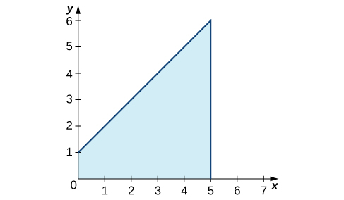
Figure $\PageIndex{10}$:The graph shows the area under the function $(x)=x+1$ over $[0,5].$

The region is a trapezoid lying on its side, so we can use the area formula for a trapezoid $A=\dfrac{1}{2}h(a+b),$ where h represents height, and a and b represent the two parallel sides. Then,

$∫^5_0x+1dx=\dfrac{1}{2}h(a+b)=\dfrac{1}{2}⋅5⋅(1+6)=\dfrac{35}{2}$.

Thus the average value of the function is

$\dfrac{1}{5−0}∫^5_0x+1dx=\dfrac{1}{5}⋅\dfrac{35}{2}=\dfrac{7}{2}$.

Exercise $\PageIndex{7}$

Find the average value of $f(x)=6−2x$ over the interval $[0,3].$

Hint: Use the average value formula, and use geometry to evaluate the integral.

Answer: 3

Key Concepts

The definite integral can be used to calculate net signed area, which is the area above the x-axis less the area below the x-axis. Net signed area can be positive, negative, or zero.
The average value of a function can be calculated using definite integrals.

Key Equations

Definite Integral

$\displaystyle∫^b_af(x)dx=\lim_{n→∞}\sum_{i=1}^nf(x^∗_i)Δx$

Glossary

average value of a function: (or $f_{ave})$ the average value of a function on an interval can be found by calculating the definite integral of the function and dividing that value by the length of the interval

variable of integration: indicates which variable you are integrating with respect to; if it is x, then the function in the integrand is followed by dx

Contributors

Gilbert Strang (MIT) and Edwin “Jed” Herman (Harvey Mudd) with many contributing authors. This content by OpenStax is licensed with a CC-BY-SA-NC 4.0 license. Download for free at http://cnx.org.

Search

Text Color

Text Size

Margin Size

Font Type