8.2E: Exercises for Direction Fields and Numerical Methods

Last updated
Save as PDF

Page ID: 18483

$ \newcommand{\vecs}[1]{\overset { \scriptstyle \rightharpoonup} {\mathbf{#1}} } $ $ \newcommand{\vecd}[1]{\overset{-\!-\!\rightharpoonup}{\vphantom{a}\smash {#1}}} $$\newcommand{\id}{\mathrm{id}}$ $ \newcommand{\Span}{\mathrm{span}}$ $ \newcommand{\kernel}{\mathrm{null}\,}$ $ \newcommand{\range}{\mathrm{range}\,}$ $ \newcommand{\RealPart}{\mathrm{Re}}$ $ \newcommand{\ImaginaryPart}{\mathrm{Im}}$ $ \newcommand{\Argument}{\mathrm{Arg}}$ $ \newcommand{\norm}[1]{\| #1 \|}$ $ \newcommand{\inner}[2]{\langle #1, #2 \rangle}$ $ \newcommand{\Span}{\mathrm{span}}$ $\newcommand{\id}{\mathrm{id}}$ $ \newcommand{\Span}{\mathrm{span}}$ $ \newcommand{\kernel}{\mathrm{null}\,}$ $ \newcommand{\range}{\mathrm{range}\,}$ $ \newcommand{\RealPart}{\mathrm{Re}}$ $ \newcommand{\ImaginaryPart}{\mathrm{Im}}$ $ \newcommand{\Argument}{\mathrm{Arg}}$ $ \newcommand{\norm}[1]{\| #1 \|}$ $ \newcommand{\inner}[2]{\langle #1, #2 \rangle}$ $ \newcommand{\Span}{\mathrm{span}}$$\newcommand{\AA}{\unicode[.8,0]{x212B}}$

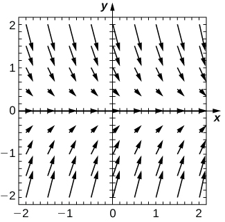
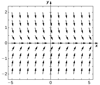
For exercises 1 - 3, use the direction field below from the differential equation $ y'=−2y.$ Sketch the graph of the solution for the given initial conditions.

$A direction field with horizontal arrows pointing to the right at 0. The arrows above the x axis point down and to the right. The further away from the x axis, the steeper the arrows are, and the closer to the x axis, the flatter the arrows are. Likewise, the arrows below the x axis point up and to the right. The further away from the x axis, the steeper the arrows are, and the closer to the x axis, the flatter the arrows are.$

1) $ y(0)=1$

2) $ y(0)=0$

Answer: $A graph of the given direction field with a flat line drawn on the axis. The arrows point up for y < 0 and down for y > 0. The closer they are to the x axis, the more horizontal the arrows are, and the further away they are, the more vertical they become.$

3) $ y(0)=−1$

4) Are there any equilibria among the solutions of the differential equation from exercises 1 - 3? List any equilibria along with their stabilities.

Answer: $ y=0$ is a stable equilibrium

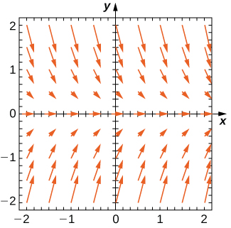
For exercises 5 - 7, use the direction field below from the differential equation $ y'=y^2−2y$. Sketch the graph of the solution for the given initial conditions.

$A direction field with horizontal arrows at y = 0 and y = 2. The arrows point up for y > 2 and for y < 0. The arrows point down for 0 < y < 2. The closer the arrows are to these lines, the more horizontal they are, and the further away, the more vertical the arrows are.$

5) $ y(0)=3$

6) $ y(0)=1$

Answer: $A direction field with horizontal arrows at y = 0 and y = 2. The arrows point up for y > 2 and for y < 0. The arrows point down for 0 < y < 2. The closer the arrows are to these lines, the more horizontal they are, and the further away, the more vertical the arrows are. A solution is sketched that follows y = 2 in quadrant two, goes through (0, 1), and then follows the x axis.$

7) $ y(0)=−1$

8) Are there any equilibria among the solutions of the differential equation from exercises 5 - 7? List any equilibria along with their stabilities.

Answer: $ y=0$ is a stable equilibrium and $ y=2$ is unstable

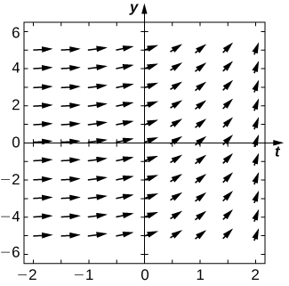
In exercises 9 - 13, draw the direction field for the following differential equations, then solve the differential equation. Draw your solution on top of the direction field. Does your solution follow along the arrows on your direction field?

9) $ y'=t^3$

10) $ y'=e^t$

Answer: $A direction field over the four quadrants. As t goes from 0 to infinity, the arrows become more and more vertical after being horizontal closer to x = 0.$

11) $ \dfrac{dy}{dx}=x^2\cos x$

12) $ \dfrac{dy}{dt}=te^t$

Answer: $A direction field over [-2, 2] in the x and y axes. The arrows point slightly down and to the right over [-2, 0] and gradually become vertical over [0, 2].$

13) $ \dfrac{dx}{dt}=\cosh(t)$

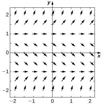
In exercises 14 - 18, draw the directional field for the following differential equations. What can you say about the behavior of the solution? Are there equilibria? What stability do these equilibria have?

14) $ y'=y^2−1$

Answer: There appear to be equlibria at $y = -1$ (stable) and $y = 1$ (unstable).
$A direction field with horizontal arrows pointing to the right at y = 1 and y = -1. The arrows point up for y < -1 and y > 1. The arrows point down for -1 < y < 1. The closer the arrows are to these lines, the more horizontal they are, and the further away they are, the more vertical they are.$

15) $ y'=y−x$

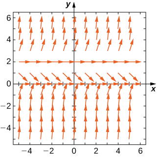
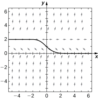
16) $ y'=1−y^2−x^2$

Answer: There do not appear to be any equilibria.
$A direction field with arrows pointing down and to the right for nearly all points in [-2, 2] on the x and y axes. Close to the origin, the arrows become more horizontal, point to the upper right, become more horizontal, and then point down to the right again.$

17) $ y'=t^2\sin y$

18) $ y'=3y+xy$

Answer: There appears to be an unstable equilibrium at $y=0.$
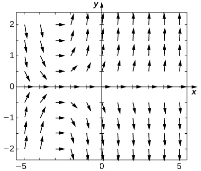
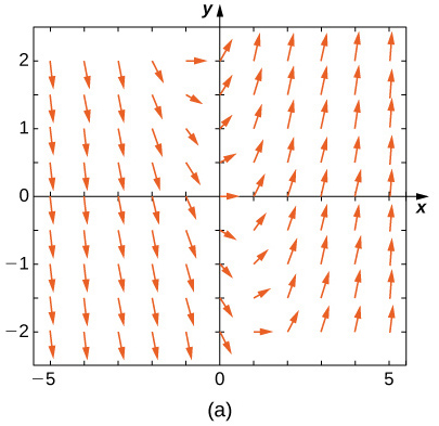
$A direction field with horizontal arrows pointing to the right on the x axis and x = -3. Above the x axis and for x < -3, the arrows point down. For x > -3, the arrows point up. Below the x axis and for x < -3, the arrows point up. For x > -3, the arrows point down. The further away from the x axis and x = -3, the arrows become more vertical, and the closer they become, the more horizontal they become.$

Match the direction field with the given differential equations. Explain your selections.

$A direction field with arrows pointing down and to the right in quadrants two and three. After crossing the y axis, the arrows change direction and point up to the right.$ $A direction field with horizontal arrows pointing to the left in quadrants two and three. In crossing the y axis, the arrows switch and point upward in quadrants one and four.$ $A direction field with horizontal arrows pointing to the right on the x axis. Above, the arrows point down and to the right, and below, the arrows point up and to the right. The further from the x axis, the more vertical the arrows become.$ $A direction field with horizontal arrows on the x and y axes. The arrows point down and to the right in quadrants one and three. They point up and to the right in quadrants two and four.$ $A direction field with arrows pointing up in quadrants two and three, to the right on the y axis, and down in quadrants one and four.$

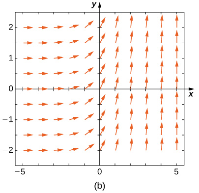
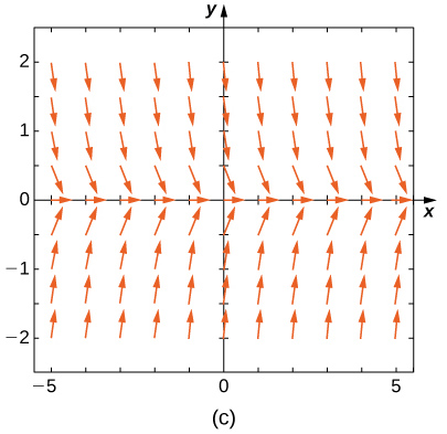
19) $ y'=−3y$

20) $ y'=−3t$

Answer: $ E$

21) $ y'=e^t$

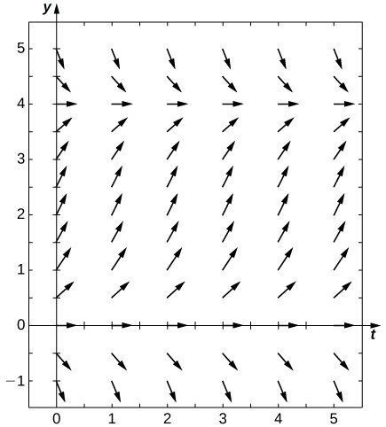
22) $ y'=\frac{1}{2}y+t$

Answer: $ A$

23) $ y'=−ty$

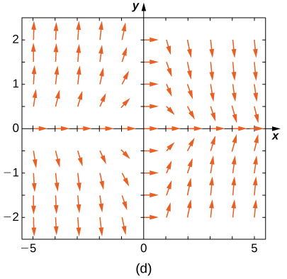
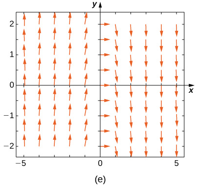
Match the direction field with the given differential equations. Explain your selections.

$A direction field with horizontal arrows pointing to the right on the x and y axes. In quadrants one and three, the arrows point up, and in quadrants two and four, they point down.$ $A direction field with horizontal arrows pointing to the right on the x and y axes. In quadrants one and three, the arrows point up and to the right, and in quadrants two and four, the arrows point down and to the right.$ $A direction field with horizontal arrows pointing to the right on the x and y axes. In quadrants two and three, the arrows point down, and in quadrants one and four, the arrows point up.$ $A direction field with horizontal arrows pointing to the right on the x axis. The arrows point up and to the right in all quadrants. The closer the arrows are to the x axis, the more horizontal the arrows are, and the further away they are, the more vertical they are.$ $A direction field with horizontal arrows on the y axis. The arrows are also more horizontal closer to y = 1.5, y = -1.5, and the y axis. For y > 1.5 and x < 0, for y < -1.5 and x < 0, and for -1.5 < y < 1.5 and x > 0-, the arrows point down. For y> 1.5 and x > 0, for y < -1.5, for y < -1.5 and x > 0, and for -1.5 < y < 1.5 and x < 0, the arrows point up.$

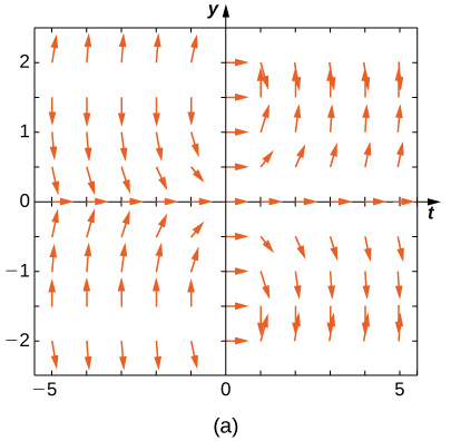
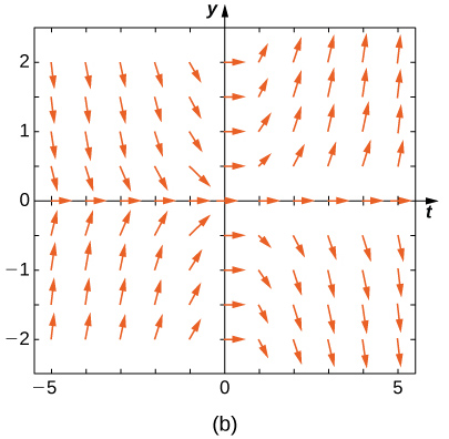
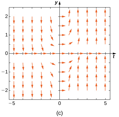
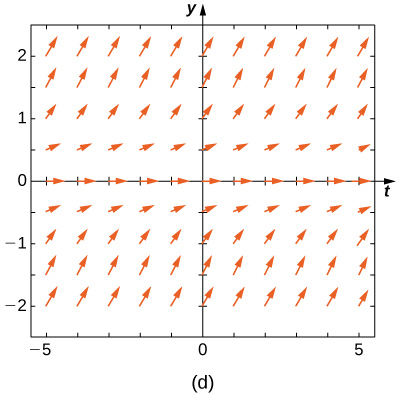
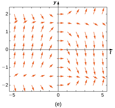
24) $ y'=t\sin y$

Answer: $ B$

25) $ y'=−t\cos y$

26) $ y'=t\tan y$

Answer: $ A$

27) $ y'=\sin^2y$

28) $ y'=y^2t^3$

Answer: $ C$

Estimate the following solutions using Euler’s method with $ n=5$ steps over the interval $ t=[0,1].$ If you are able to solve the initial-value problem exactly, compare your solution with the exact solution. If you are unable to solve the initial-value problem, the exact solution will be provided for you to compare with Euler’s method. How accurate is Euler’s method?

29) $ y'=−3y,\quad y(0)=1$

30) $ y'=t^2,\quad y(0)=1$

Answer: $ 2.24,$ exact: $ 3$

Solution:

31) $ y′=3t−y,\quad y(0)=1.$ Exact solution is $ y=3t+4e^{−t}−3$

32) $ y′=y+t^2,\quad y(0)=3.$ Exact solution is $ y=5e^t−2−t^2−2t$

Answer: $ 7.739364,$ exact: $ 5(e−1)$

33) $ y′=2t,\quad y(0)=0$

34) [T] $ y'=e^{x+y},y(0)=−1.$ Exact solution is $ y=−\ln(e+1−e^x)$

Answer: $ −0.2535,$ exact: $ 0$

35) $ y′=y^2\ln(x+1),\quad y(0)=1.$ Exact solution is $ y=−\dfrac{1}{(x+1)(\ln(x+1)−1)}$

36) $ y′=2^x,\quad y(0)=0.$ Exact solution is $ y=\dfrac{2^x−1}{\ln 2}$

Answer: $ 1.345,$ exact: $ \frac{1}{\ln(2)}$

37) $ y′=y,\quad y(0)=−1.$ Exact solution is $ y=−e^x$.

38) $ y′=−5t,\quad y(0)=−2.$ Exact solution is $ y=−\frac{5}{2}t^2−2$

Answer: $ −4,$ exact: $ −1/2$

Differential equations can be used to model disease epidemics. In the next set of problems, we examine the change of size of two sub-populations of people living in a city: individuals who are infected and individuals who are susceptible to infection. $ S$ represents the size of the susceptible population, and $ I$ represents the size of the infected population. We assume that if a susceptible person interacts with an infected person, there is a probability $ c$ that the susceptible person will become infected. Each infected person recovers from the infection at a rate $ r$ and becomes susceptible again. We consider the case of influenza, where we assume that no one dies from the disease, so we assume that the total population size of the two sub-populations is a constant number, $ N$. The differential equations that model these population sizes are

$ S'=rI−cSI$ and $ I'=cSI−rI.$

Here $ c$ represents the contact rate and $ r$ is the recovery rate.

39) Show that, by our assumption that the total population size is constant $ (S+I=N),$ you can reduce the system to a single differential equation in $ I:I'=c(N−I)I−rI.$

40) Assuming the parameters are $ c=0.5,N=5,$ and $ r=0.5$, draw the resulting directional field.

Answer: $A direction field with horizontal arrows pointing to the right on the x axis and at y = 4. The arrows below the x axis and above y = 4 point down and to the right. The arrows between the x axis and y = 4 point up and to the right.$

41) [T] Use computational software or a calculator to compute the solution to the initial-value problem $ y'=ty,y(0)=2$ using Euler’s Method with the given step size $ h$. Find the solution at $ t=1$. For a hint, here is “pseudo-code” for how to write a computer program to perform Euler’s Method for $ y'=f(t,y),y(0)=2:$

Create function $ f(t,y)$

Define parameters $ y(1)=y_0,t(0)=0,$ step size $ h$, and total number of steps, $ N$

Write a for-loop:

for $ k=1$ to $ N$

$ fn=f(t(k),y(k))$

$ y(k+1)=y(k)+h*fn$

$ t(k+1)=t(k)+h$

42) Solve the initial-value problem for the exact solution.

Answer: $ y'=2e^{t^2/2}$

43) Draw the directional field

44) $ h=1$

Answer: $ 2$

45) [T] $ h=10$

46) [T] $ h=100$

Answer: $ 3.2756$

47) [T] $ h=1000$

48) [T] Evaluate the exact solution at $ t=1$. Make a table of errors for the relative error between the Euler’s method solution and the exact solution. How much does the error change? Can you explain?

Answer

Exact solution: y =$ 2\sqrt{e}.$

Step Size	Error
$ h=1$	$ 0.3935$
$ h=10$	$ 0.06163$
$ h=100$	$ 0.006612$
$ h=10000$	$ 0.0006661$

For exercises 49 - 53, consider the initial-value problem $ y'=−2y,$ with $y(0)=2.$

49) Show that $ y=2e^{−2x}$ solves this initial-value problem.

50) Draw the directional field of this differential equation.

Answer: $Direction field for the differential equation y' = -2y. A direction field with horizontal arrows pointing to the right on the x-axis. Above the x-axis, the arrows point down and to the right. Below the x axis, the arrows point up and to the right. The closer the arrows are to the x-axis, the more horizontal the arrows are, and the further away they are from the x-axis, the more vertical the arrows are.$

51) [T] By hand or by calculator or computer, approximate the solution using Euler’s Method at $ t=10$ using $ h=5$.

52) [T] By calculator or computer, approximate the solution using Euler’s Method at $ t=10$ using $ h=100.$

Answer: $ 4.0741e^{−10}$

53) [T] Plot exact answer and each Euler approximation (for $ h=5$ and $ h=100$) at each h on the directional field. What do you notice?

Step Size	Error
\( h=1\)	\( 0.3935\)
\( h=10\)	\( 0.06163\)
\( h=100\)	\( 0.006612\)
\( h=10000\)	\( 0.0006661\)