Mathematics LibreTexts

13.9E: Optimization of Functions of Several Variables (Exercises)

  • Page ID
    25315
  • \( \newcommand{\vecs}[1]{\overset { \scriptstyle \rightharpoonup} {\mathbf{#1}} } \)

    \( \newcommand{\vecd}[1]{\overset{-\!-\!\rightharpoonup}{\vphantom{a}\smash {#1}}} \)

    \( \newcommand{\id}{\mathrm{id}}\) \( \newcommand{\Span}{\mathrm{span}}\)

    ( \newcommand{\kernel}{\mathrm{null}\,}\) \( \newcommand{\range}{\mathrm{range}\,}\)

    \( \newcommand{\RealPart}{\mathrm{Re}}\) \( \newcommand{\ImaginaryPart}{\mathrm{Im}}\)

    \( \newcommand{\Argument}{\mathrm{Arg}}\) \( \newcommand{\norm}[1]{\| #1 \|}\)

    \( \newcommand{\inner}[2]{\langle #1, #2 \rangle}\)

    \( \newcommand{\Span}{\mathrm{span}}\)

    \( \newcommand{\id}{\mathrm{id}}\)

    \( \newcommand{\Span}{\mathrm{span}}\)

    \( \newcommand{\kernel}{\mathrm{null}\,}\)

    \( \newcommand{\range}{\mathrm{range}\,}\)

    \( \newcommand{\RealPart}{\mathrm{Re}}\)

    \( \newcommand{\ImaginaryPart}{\mathrm{Im}}\)

    \( \newcommand{\Argument}{\mathrm{Arg}}\)

    \( \newcommand{\norm}[1]{\| #1 \|}\)

    \( \newcommand{\inner}[2]{\langle #1, #2 \rangle}\)

    \( \newcommand{\Span}{\mathrm{span}}\) \( \newcommand{\AA}{\unicode[.8,0]{x212B}}\)

    \( \newcommand{\vectorA}[1]{\vec{#1}}      % arrow\)

    \( \newcommand{\vectorAt}[1]{\vec{\text{#1}}}      % arrow\)

    \( \newcommand{\vectorB}[1]{\overset { \scriptstyle \rightharpoonup} {\mathbf{#1}} } \)

    \( \newcommand{\vectorC}[1]{\textbf{#1}} \)

    \( \newcommand{\vectorD}[1]{\overrightarrow{#1}} \)

    \( \newcommand{\vectorDt}[1]{\overrightarrow{\text{#1}}} \)

    \( \newcommand{\vectE}[1]{\overset{-\!-\!\rightharpoonup}{\vphantom{a}\smash{\mathbf {#1}}}} \)

    \( \newcommand{\vecs}[1]{\overset { \scriptstyle \rightharpoonup} {\mathbf{#1}} } \)

    \( \newcommand{\vecd}[1]{\overset{-\!-\!\rightharpoonup}{\vphantom{a}\smash {#1}}} \)

    \(\newcommand{\avec}{\mathbf a}\) \(\newcommand{\bvec}{\mathbf b}\) \(\newcommand{\cvec}{\mathbf c}\) \(\newcommand{\dvec}{\mathbf d}\) \(\newcommand{\dtil}{\widetilde{\mathbf d}}\) \(\newcommand{\evec}{\mathbf e}\) \(\newcommand{\fvec}{\mathbf f}\) \(\newcommand{\nvec}{\mathbf n}\) \(\newcommand{\pvec}{\mathbf p}\) \(\newcommand{\qvec}{\mathbf q}\) \(\newcommand{\svec}{\mathbf s}\) \(\newcommand{\tvec}{\mathbf t}\) \(\newcommand{\uvec}{\mathbf u}\) \(\newcommand{\vvec}{\mathbf v}\) \(\newcommand{\wvec}{\mathbf w}\) \(\newcommand{\xvec}{\mathbf x}\) \(\newcommand{\yvec}{\mathbf y}\) \(\newcommand{\zvec}{\mathbf z}\) \(\newcommand{\rvec}{\mathbf r}\) \(\newcommand{\mvec}{\mathbf m}\) \(\newcommand{\zerovec}{\mathbf 0}\) \(\newcommand{\onevec}{\mathbf 1}\) \(\newcommand{\real}{\mathbb R}\) \(\newcommand{\twovec}[2]{\left[\begin{array}{r}#1 \\ #2 \end{array}\right]}\) \(\newcommand{\ctwovec}[2]{\left[\begin{array}{c}#1 \\ #2 \end{array}\right]}\) \(\newcommand{\threevec}[3]{\left[\begin{array}{r}#1 \\ #2 \\ #3 \end{array}\right]}\) \(\newcommand{\cthreevec}[3]{\left[\begin{array}{c}#1 \\ #2 \\ #3 \end{array}\right]}\) \(\newcommand{\fourvec}[4]{\left[\begin{array}{r}#1 \\ #2 \\ #3 \\ #4 \end{array}\right]}\) \(\newcommand{\cfourvec}[4]{\left[\begin{array}{c}#1 \\ #2 \\ #3 \\ #4 \end{array}\right]}\) \(\newcommand{\fivevec}[5]{\left[\begin{array}{r}#1 \\ #2 \\ #3 \\ #4 \\ #5 \\ \end{array}\right]}\) \(\newcommand{\cfivevec}[5]{\left[\begin{array}{c}#1 \\ #2 \\ #3 \\ #4 \\ #5 \\ \end{array}\right]}\) \(\newcommand{\mattwo}[4]{\left[\begin{array}{rr}#1 \amp #2 \\ #3 \amp #4 \\ \end{array}\right]}\) \(\newcommand{\laspan}[1]{\text{Span}\{#1\}}\) \(\newcommand{\bcal}{\cal B}\) \(\newcommand{\ccal}{\cal C}\) \(\newcommand{\scal}{\cal S}\) \(\newcommand{\wcal}{\cal W}\) \(\newcommand{\ecal}{\cal E}\) \(\newcommand{\coords}[2]{\left\{#1\right\}_{#2}}\) \(\newcommand{\gray}[1]{\color{gray}{#1}}\) \(\newcommand{\lgray}[1]{\color{lightgray}{#1}}\) \(\newcommand{\rank}{\operatorname{rank}}\) \(\newcommand{\row}{\text{Row}}\) \(\newcommand{\col}{\text{Col}}\) \(\renewcommand{\row}{\text{Row}}\) \(\newcommand{\nul}{\text{Nul}}\) \(\newcommand{\var}{\text{Var}}\) \(\newcommand{\corr}{\text{corr}}\) \(\newcommand{\len}[1]{\left|#1\right|}\) \(\newcommand{\bbar}{\overline{\bvec}}\) \(\newcommand{\bhat}{\widehat{\bvec}}\) \(\newcommand{\bperp}{\bvec^\perp}\) \(\newcommand{\xhat}{\widehat{\xvec}}\) \(\newcommand{\vhat}{\widehat{\vvec}}\) \(\newcommand{\uhat}{\widehat{\uvec}}\) \(\newcommand{\what}{\widehat{\wvec}}\) \(\newcommand{\Sighat}{\widehat{\Sigma}}\) \(\newcommand{\lt}{<}\) \(\newcommand{\gt}{>}\) \(\newcommand{\amp}{&}\) \(\definecolor{fillinmathshade}{gray}{0.9}\)

    Absolute Extrema on Closed and Bounded Regions

    In exercises 1 - 4, find the absolute extrema of the given function on the indicated closed and bounded set \( R\).

    1) \( f(x,y)=xy−x−3y; R\) is the triangular region with vertices \( (0,0),(0,4),\) and \( (5,0)\).

    2) Find the absolute maximum and minimum values of \( f(x,y)=x^2+y^2−2y+1\) on the region \( R=\{(x,y)∣x^2+y^2≤4\}.\)

    Answer:
    \(f\) has an absolute minimum of \(0\) at \( (0, 1) \) and an absolute maximum of \(9\) at \( (0,−2)\).

    3) \( f(x,y)=x^3−3xy−y^3\) on \( R=\{(x,y):−2≤x≤2,−2≤y≤2\}\)

    4) \( f(x,y)=\frac{−2y}{x^2+y^2+1}\) on \( R=\{(x,y):x^2+y^2≤4\}\)

    Answer:
    \(f\) has an absolute minimum of \( -1\) at \( (0,1)\) and an absolute maximum of \( 1\) at \( (0,−1)\).

    5)  To be created...

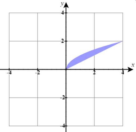
    6) Find the absolute minimum and absolute maximum of the function \(f(x,y) = xy^2 - 2x + 3\) on the region between \(y = x/2\) and \(y = \sqrt{x}\), for \(0 \le x \le 4\), showing all work, including work to find any critical points of \(f\).  See the plot of the region in the \(xy\)-plane below.

    clipboard_ebd2efe5743e6ab99eb257f054b7c93d6.png
    Figure \(\PageIndex{1}\): Closed and bounded region in the \(xy\)-plane for Problem 6.
    Answer:
    \(f\) has an absolute minimum of   \( 3 - \frac{8\sqrt{6}}{9} \approx 0.822676\)   at \( \left( \frac{2\sqrt{6}}{3}, \frac{\sqrt{6}}{3} \right)\) and an absolute maximum of \( 11\) at \( (4, 2)\).
     

    Figure \(\PageIndex{2}\): The top surface of this solid represents the portion of the surface plot of \(f\) restricted to be above the given region in the \(xy\)-plane.
    Solution:
    First, we find the critical points of \(f\).  The partials of \(f\) are:
    \[\begin{align*} f_x(x,y) &= y^2 - 2 \\ f_y(x,y) &= 2xy \end{align*}\]
    Setting the partials both equal to \(0\), we get the equations:
    \[y^2 - 2 = 0  \qquad \text{and}  \qquad 2xy = 0 \nonumber\]
    Solving the first for \(y\) gives us: \( y = \pm \sqrt{2}\).

    If \(y = \sqrt{2}\), the second equation becomes \(2x(\sqrt{2}) = 0\).  Solving this equation for \(x\), we get \(x = 0\).

    Note that if \(y = -\sqrt{2}\), we also get \(x = 0\).

    Thus, the critical points of \(f\) are: \( (0, -\sqrt{2})\) and \( (0, \sqrt{2}) \).

    Since neither of these critical points is inside the closed, bounded region we are looking at in this problem, we can reject them as locations of absolute extrema of \(f\) on this region.

    Now let's consider the two boundary curves, remembering to check the endpoints of the interval as we do this.

    If \(y = \sqrt{x}\), we get the function of one variable, \[\begin{align*} g(x) = f(x, \sqrt{x}) &= x (\sqrt{x})^2 - 2x + 3 \\ &= x^2 - 2x + 3 \end{align*}\]
    Now let's locate any critical values for this function \(g\).
    \[\text{Set }g'(x) = 2x  -2 =0. \nonumber\]
    Then \(x = 1\) is a critical value of \(g\).

    Since \(x = 1\) is in the interval \( [0, 4] \), we evaluate \(g\) at this critical value and at the endpoints of the interval, \(x = 0\) and \(x = 4\).
    \[\begin{align*} g(1) &= f(1, 1) = 1(1)^2 - 2(1) + 3 = \boxed{2} \\[5pt]
    g(0) &= f(0, 0) = 0(0)^2 - 2(0) + 3 =\boxed{ 3 }\\[5pt]
    g(4) &= f(4, 2) = 4(2)^2 -2(4) + 3 = \boxed{ 11 } \end{align*}\]
    Now, if \(y = x/2\), we get the function of one variable, \[\begin{align*} h(x) = f(x, \tfrac{x}{2}) &= x \left(\tfrac{x}{2}\right)^2 - 2x + 3 \\ &= \frac{x^3}{4} - 2x + 3 \end{align*}\]
    Locating any critical values for this function \(h\), we
    \[\text{Set }h'(x) = \frac{3x^2}{4}  -2 =0. \nonumber\]
    Solving this equation for \(x\), we solve as follows. \[\begin{align*}  3x^2 &= 8 \\[5pt] x^2 &= \frac{8}{3}\\[5pt] x &= \pm \sqrt{\frac{8}{3}} = \pm \frac{2\sqrt{6}}{3} \end{align*}\]
    Thus \(h\) has two critical values:  \(x = -\frac{2\sqrt{6}}{3}\) and \(x = \frac{2\sqrt{6}}{3} \approx 1.633\).

    Since the negative critical number is not in the interval \( [0, 4] \), we can reject it.  But the positive critical number is in this interval, so we evaluate \(h\) at this value.
    \[\begin{align*} h\left(\frac{2\sqrt{6}}{3}\right) &= f\left(\frac{2\sqrt{6}}{3}, \frac{\sqrt{6}}{3} \right) = \frac{2\sqrt{6}}{3}\left(\frac{\sqrt{6}}{3}\right)^2 - 2\left(\frac{2\sqrt{6}}{3}\right) + 3 \\[5pt]
    &= \frac{4\sqrt{6}}{9} - \frac{4\sqrt{6}}{3} + 3 =  \boxed{3 - \frac{8\sqrt{6}}{9}} \approx 0.822676 \\[5pt]
    h(0) &= f(0, 0) = 0(0)^2 - 2(0) + 3 = \boxed{ 3 } \\[5pt]
    h(4) &= f(4, 2) = 4(2)^2 -2(4) + 3 = \boxed{ 11 } \end{align*}\]
    Comparing the values of \(f\) at all these points, we find that:

    \(f\) has an absolute minimum of   \( 3 - \frac{8\sqrt{6}}{9} \approx 0.822676\)   at \( \left( \frac{2\sqrt{6}}{3}, \frac{\sqrt{6}}{3} \right)\) and an absolute maximum of \( 11\) at \( (4, 2)\).


    Applications

    7) Find three positive numbers the sum of which is \( 27\), such that the sum of their squares is as small as possible.

    8) Find the points on the surface \( x^2−yz=5\) that are closest to the origin.

    Hint:
    Use the distance formula. But note that you can leave off the square root, since the minimum value of the square of the distance will also minimize the distance.
    Answer:
    \( (\sqrt{5},0,0),(−\sqrt{5},0,0)\)

    9) Find the maximum volume of a rectangular box with three faces in the coordinate planes and a vertex in the first octant on the plane \(x+y+z=1\).

    10) The sum of the length and the girth (perimeter of a cross-section) of a package carried by a delivery service cannot exceed \(108\) in. Find the dimensions of the rectangular package of largest volume that can be sent.

    Answer:
    \( 18\) in. by \( 36\) in. by \( 18\) in.

    11) A cardboard box without a lid is to be made with a volume of \( 4\) ft3. Find the dimensions of the box that requires the least amount of cardboard.

    12) Find the point on the surface \( f(x,y)=x^2+y^2+10\) nearest the plane \( x+2y−z=0.\) Identify the point on the plane.

    Hint:
    Here one approach is the find the distance between a point \((x_0, y_0, z_0)\) on the surface and the plane, using what you learned in Section 11.5. Then you can substitute the surface function into this distance function for \(z_0\) and substitute \(x\) for \(x_0\) and \(y\) for \(y_0\). This will give you a function of \(x\) and \(y\) that you can minimize.
    Answer:
    \( (0.5,1,11.25)\) is the point on the surface nearest the plane.
    Although it was not requested, note that \( (\frac{47}{24},\frac{47}{12},\frac{235}{24})\) is the point on the plane that is nearest the surface.
    See this problem illustrated in CalcPlot3D.

    13) Find the point in the plane \( 2x−y+2z=16\) that is closest to the origin.

    14) A company manufactures two types of athletic shoes: jogging shoes and cross-trainers. The total revenue from \( x\) units of jogging shoes and \( y\) units of cross-trainers is given by \( R(x,y)=−5x^2−8y^2−2xy+42x+102y,\) where \( x\) and \( y\) are in thousands of units. Find the values of \( x\) and \( y\) to maximize the total revenue.

    Answer:
    \( x=3\) and \( y=6\)

    15) A shipping company handles rectangular boxes provided the sum of the length, width, and height of the box does not exceed \( 96\)in. Find the dimensions of the box that meets this condition and has the largest volume.

    16) Find the maximum volume of a cylindrical soda can such that the sum of its height and circumference is \( 120\) cm.

    Answer:
    \( V=\frac{64,000}{π}\,\text{cm}^3≈20,372\,\text{cm}^3\)


    Contributors

    • Gilbert Strang (MIT) and Edwin “Jed” Herman (Harvey Mudd) with many contributing authors. This content by OpenStax is licensed with a CC-BY-SA-NC 4.0 license. Download for free at http://cnx.org.

    • Paul Seeburger (Monroe Community College) edited the LaTeX , added all of Problem 6 and added Hints to Problems 8 and 12 and expanded the Answer to problem 12.

    13.9E: Optimization of Functions of Several Variables (Exercises) is shared under a CC BY-NC-SA license and was authored, remixed, and/or curated by LibreTexts.

    • Was this article helpful?