
2.7: Limit of Trigonometric functions
- Page ID
- 10283
This page is a draft and is under active development.
\( \newcommand{\vecs}[1]{\overset { \scriptstyle \rightharpoonup} {\mathbf{#1}} } \)
\( \newcommand{\vecd}[1]{\overset{-\!-\!\rightharpoonup}{\vphantom{a}\smash {#1}}} \)
\( \newcommand{\dsum}{\displaystyle\sum\limits} \)
\( \newcommand{\dint}{\displaystyle\int\limits} \)
\( \newcommand{\dlim}{\displaystyle\lim\limits} \)
\( \newcommand{\id}{\mathrm{id}}\) \( \newcommand{\Span}{\mathrm{span}}\)
( \newcommand{\kernel}{\mathrm{null}\,}\) \( \newcommand{\range}{\mathrm{range}\,}\)
\( \newcommand{\RealPart}{\mathrm{Re}}\) \( \newcommand{\ImaginaryPart}{\mathrm{Im}}\)
\( \newcommand{\Argument}{\mathrm{Arg}}\) \( \newcommand{\norm}[1]{\| #1 \|}\)
\( \newcommand{\inner}[2]{\langle #1, #2 \rangle}\)
\( \newcommand{\Span}{\mathrm{span}}\)
\( \newcommand{\id}{\mathrm{id}}\)
\( \newcommand{\Span}{\mathrm{span}}\)
\( \newcommand{\kernel}{\mathrm{null}\,}\)
\( \newcommand{\range}{\mathrm{range}\,}\)
\( \newcommand{\RealPart}{\mathrm{Re}}\)
\( \newcommand{\ImaginaryPart}{\mathrm{Im}}\)
\( \newcommand{\Argument}{\mathrm{Arg}}\)
\( \newcommand{\norm}[1]{\| #1 \|}\)
\( \newcommand{\inner}[2]{\langle #1, #2 \rangle}\)
\( \newcommand{\Span}{\mathrm{span}}\) \( \newcommand{\AA}{\unicode[.8,0]{x212B}}\)
\( \newcommand{\vectorA}[1]{\vec{#1}} % arrow\)
\( \newcommand{\vectorAt}[1]{\vec{\text{#1}}} % arrow\)
\( \newcommand{\vectorB}[1]{\overset { \scriptstyle \rightharpoonup} {\mathbf{#1}} } \)
\( \newcommand{\vectorC}[1]{\textbf{#1}} \)
\( \newcommand{\vectorD}[1]{\overrightarrow{#1}} \)
\( \newcommand{\vectorDt}[1]{\overrightarrow{\text{#1}}} \)
\( \newcommand{\vectE}[1]{\overset{-\!-\!\rightharpoonup}{\vphantom{a}\smash{\mathbf {#1}}}} \)
\( \newcommand{\vecs}[1]{\overset { \scriptstyle \rightharpoonup} {\mathbf{#1}} } \)
\(\newcommand{\longvect}{\overrightarrow}\)
\( \newcommand{\vecd}[1]{\overset{-\!-\!\rightharpoonup}{\vphantom{a}\smash {#1}}} \)
\(\newcommand{\avec}{\mathbf a}\) \(\newcommand{\bvec}{\mathbf b}\) \(\newcommand{\cvec}{\mathbf c}\) \(\newcommand{\dvec}{\mathbf d}\) \(\newcommand{\dtil}{\widetilde{\mathbf d}}\) \(\newcommand{\evec}{\mathbf e}\) \(\newcommand{\fvec}{\mathbf f}\) \(\newcommand{\nvec}{\mathbf n}\) \(\newcommand{\pvec}{\mathbf p}\) \(\newcommand{\qvec}{\mathbf q}\) \(\newcommand{\svec}{\mathbf s}\) \(\newcommand{\tvec}{\mathbf t}\) \(\newcommand{\uvec}{\mathbf u}\) \(\newcommand{\vvec}{\mathbf v}\) \(\newcommand{\wvec}{\mathbf w}\) \(\newcommand{\xvec}{\mathbf x}\) \(\newcommand{\yvec}{\mathbf y}\) \(\newcommand{\zvec}{\mathbf z}\) \(\newcommand{\rvec}{\mathbf r}\) \(\newcommand{\mvec}{\mathbf m}\) \(\newcommand{\zerovec}{\mathbf 0}\) \(\newcommand{\onevec}{\mathbf 1}\) \(\newcommand{\real}{\mathbb R}\) \(\newcommand{\twovec}[2]{\left[\begin{array}{r}#1 \\ #2 \end{array}\right]}\) \(\newcommand{\ctwovec}[2]{\left[\begin{array}{c}#1 \\ #2 \end{array}\right]}\) \(\newcommand{\threevec}[3]{\left[\begin{array}{r}#1 \\ #2 \\ #3 \end{array}\right]}\) \(\newcommand{\cthreevec}[3]{\left[\begin{array}{c}#1 \\ #2 \\ #3 \end{array}\right]}\) \(\newcommand{\fourvec}[4]{\left[\begin{array}{r}#1 \\ #2 \\ #3 \\ #4 \end{array}\right]}\) \(\newcommand{\cfourvec}[4]{\left[\begin{array}{c}#1 \\ #2 \\ #3 \\ #4 \end{array}\right]}\) \(\newcommand{\fivevec}[5]{\left[\begin{array}{r}#1 \\ #2 \\ #3 \\ #4 \\ #5 \\ \end{array}\right]}\) \(\newcommand{\cfivevec}[5]{\left[\begin{array}{c}#1 \\ #2 \\ #3 \\ #4 \\ #5 \\ \end{array}\right]}\) \(\newcommand{\mattwo}[4]{\left[\begin{array}{rr}#1 \amp #2 \\ #3 \amp #4 \\ \end{array}\right]}\) \(\newcommand{\laspan}[1]{\text{Span}\{#1\}}\) \(\newcommand{\bcal}{\cal B}\) \(\newcommand{\ccal}{\cal C}\) \(\newcommand{\scal}{\cal S}\) \(\newcommand{\wcal}{\cal W}\) \(\newcommand{\ecal}{\cal E}\) \(\newcommand{\coords}[2]{\left\{#1\right\}_{#2}}\) \(\newcommand{\gray}[1]{\color{gray}{#1}}\) \(\newcommand{\lgray}[1]{\color{lightgray}{#1}}\) \(\newcommand{\rank}{\operatorname{rank}}\) \(\newcommand{\row}{\text{Row}}\) \(\newcommand{\col}{\text{Col}}\) \(\renewcommand{\row}{\text{Row}}\) \(\newcommand{\nul}{\text{Nul}}\) \(\newcommand{\var}{\text{Var}}\) \(\newcommand{\corr}{\text{corr}}\) \(\newcommand{\len}[1]{\left|#1\right|}\) \(\newcommand{\bbar}{\overline{\bvec}}\) \(\newcommand{\bhat}{\widehat{\bvec}}\) \(\newcommand{\bperp}{\bvec^\perp}\) \(\newcommand{\xhat}{\widehat{\xvec}}\) \(\newcommand{\vhat}{\widehat{\vvec}}\) \(\newcommand{\uhat}{\widehat{\uvec}}\) \(\newcommand{\what}{\widehat{\wvec}}\) \(\newcommand{\Sighat}{\widehat{\Sigma}}\) \(\newcommand{\lt}{<}\) \(\newcommand{\gt}{>}\) \(\newcommand{\amp}{&}\) \(\definecolor{fillinmathshade}{gray}{0.9}\)Trigonometric function an Introduction
Radian Measure
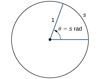
To use trigonometric functions, we first must understand how to measure the angles. Although we can use both radians and degrees, \(radians\) are a more natural measurement because they are related directly to the unit circle, a circle with radius 1. The radian measure of an angle is defined as follows. Given an angle \(θ\), let \(s\) be the length of the corresponding arc on the unit circle (Figure). We say the angle corresponding to the arc of length 1 has radian measure 1.
Since an angle of \(360°\) corresponds to the circumference of a circle, or an arc of length \(2π\), we conclude that an angle with a degree measure of \(360°\) has a radian measure of \(2π\). Similarly, we see that \(180°\) is equivalent to \(\pi\) radians. Table shows the relationship between common degree and radian values.
The Six Basic Trigonometric Functions
Trigonometric functions allow us to use angle measures, in radians or degrees, to find the coordinates of a point on any circle—not only on a unit circle—or to find an angle given a point on a circle. They also define the relationship among the sides and angles of a triangle.
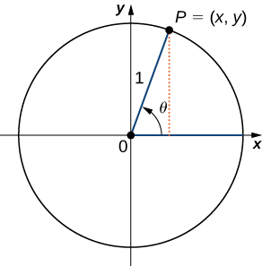
To define the trigonometric functions, first consider the unit circle centered at the origin and a point \(P=(x,y)\) on the unit circle. Let \(θ\) be an angle with an initial side that lies along the positive \(x\)-axis and with a terminal side that is the line segment \(OP\). An angle in this position is said to be in standard position (Figure \(\PageIndex{2}\)). We can then define the values of the six trigonometric functions for \(θ\) in terms of the coordinates \(x\) and \(y\).
Definition: Trigonometric functions
Let \(P=(x,y)\) be a point on the unit circle centered at the origin \(O\). Let \(θ\) be an angle with an initial side along the positive \(x\)-axis and a terminal side given by the line segment \(OP\). The trigonometric functions are then defined as
| \(\sin θ=y\) | \(cscθ=\dfrac{1}{y}\) |
| \(\cos θ=x\) | \(secθ=\dfrac{1}{x}\) |
| \(\tan θ=\dfrac{y}{x}\) | \(\cot θ=\dfrac{x}{y}\) |
If \(x=0, secθ\) and \(\tan θ\) are undefined. If \(y=0\), then \(\cot θ\) and \(cscθ\) are undefined.
We can see that for a point \(P=(x,y)\) on a circle of radius \(r\) with a corresponding angle \(θ\), the coordinates \(x\) and \(y\) satisfy
\[\begin{align} \cos θ &=\dfrac{x}{r} \\ x&=r\cos θ \end{align}\]
and
\[\begin{align} \sin θ&=\dfrac{y}{r} \\ y&=r\sin θ. \end{align}\]
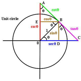
Figure \(\PageIndex{3.1}\): Diagram demonstrating trigonometric functions in the unit circle., \).
The values of the other trigonometric functions can be expressed in terms of \(x,y\), and \(r\) (Figure \(\PageIndex{3}\)).
Figure \(\PageIndex{3.2}\): For a point \(P=(x,y)\) on a circle of radius \(r\), the coordinates \(x\) and y satisfy \(x=r\cos θ\) and \(y=r\sin θ\).
Table shows the values of sine and cosine at the major angles in the first quadrant. From this table, we can determine the values of sine and cosine at the corresponding angles in the other quadrants. The values of the other trigonometric functions are calculated easily from the values of \(\sin θ\) and \(\cos θ.\)
| \(θ\)θ | \(\sin θ\) | \(\cos θ\) |
|---|---|---|
| 0 | 0 | 1 |
| \(\dfrac{π}{6}\) | \(\dfrac{1}{2}\) | \(\dfrac{\sqrt{3}}{2}\) |
| \(\dfrac{π}{4}\) | \(\dfrac{\sqrt{2}}{2}\) | \(\dfrac{\sqrt{2}}{2}\) |
| \(\dfrac{π}{3}\) | \(\dfrac{\sqrt{3}}{2}\) | \(\dfrac{1}{2}\) |
| \(\dfrac{π}{2}\) | 1 | 0 |
Example \(\PageIndex{2}\): Evaluating Trigonometric Functions
Evaluate each of the following expressions.
- \(\sin(\dfrac{2π}{3})\)
- \(\cos(−\dfrac{5π}{6})\)
- \(\tan(\dfrac{15π}{4})\)
Solution:
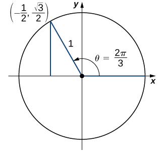
a) On the unit circle, the angle \(θ=\dfrac{2π}{3}\) corresponds to the point \((−\dfrac{1}{2},\dfrac{\sqrt{3}}{2})\). Therefore, \(sin\)(\(\dfrac{2π}{3})\)=\(y\)=\(\dfrac{\sqrt{3}}{2}\).
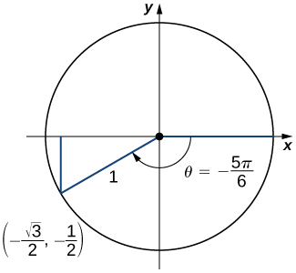
b) An angle \(θ=−\dfrac{5π}{6}\) corresponds to a revolution in the negative direction, as shown. Therefore, \(cos(−\dfrac{5π}{6})\)=\(x\)=\(−\dfrac{\sqrt{3}}{2}\).
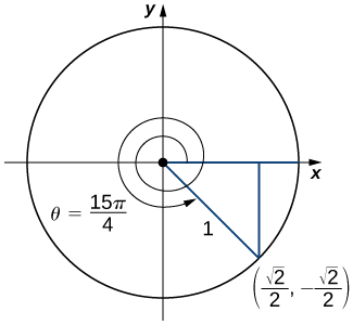
c) An angle \(θ\)=\(\dfrac{15π}{4}\)=\(2π\)+\(\dfrac{7π}{4}\). Therefore, this angle corresponds to more than one revolution, as shown. Knowing the fact that an angle of \(\dfrac{7π}{4}\) corresponds to the point \((\dfrac{\sqrt{2}}{2},\dfrac{\sqrt{2}}{2})\), we can conclude that \(tan(\dfrac{15π}{4})=\dfrac{y}{x}=−1\).
Exercise \(\PageIndex{2}\)
Evaluate \(\cos(3π/4)\) and \(\sin(−π/6)\).
- Hint
-
Look at angles on the unit circle.
- Answer
Trigonometric Identities
A trigonometric identity is an equation involving trigonometric functions that is true for all angles \(θ\) for which the functions are defined. We can use the identities to help us solve or simplify equations. The main trigonometric identities are listed next.
Rule: Trigonometric Identities
Reciprocal identities
\[\tan θ=\dfrac{\sin θ}{\cos θ}\]
\[\cot θ=\dfrac{\cos θ}{\sin θ}\]
\[csc θ=\dfrac{1}{\sin θ}\]
\[sec θ=\dfrac{1}{\cos θ}\]
Pythagorean identities
\[\sin^2θ+\cos^2θ=1\]
\[1+\tan^2θ=sec^2θ \]
\[1+\cot^2θ=csc^2θ\]
Addition and subtraction formulas
\[\sin(α±β)=\sin α\cos β±\cos α sin β\]
\[\cos(α±β)=\cos α\cos β∓\sin α \sin β\]
Double-angle formulas
\[\sin(2θ)=2\sin θ\cos θ\]
\[\cos(2θ)=2\cos^2θ−1=1−2\sin^2θ=\cos^2θ−\sin^2θ\]
Graphs and Periods of the Trigonometric Functions
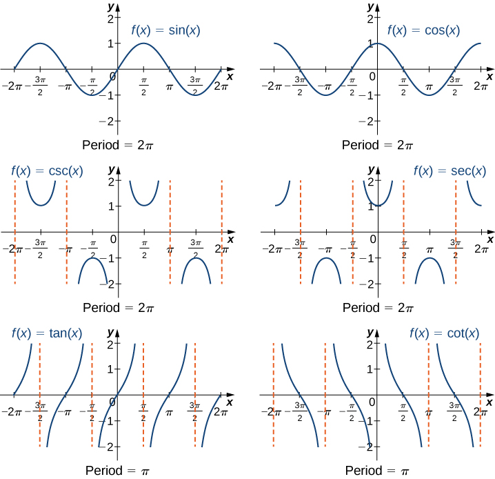
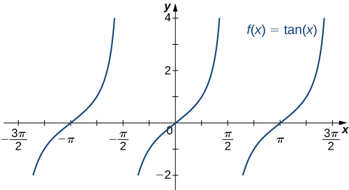
We have seen that as we travel around the unit circle, the values of the trigonometric functions repeat. We can see this pattern in the graphs of the functions. Let \(P=(x,y)\) be a point on the unit circle and let θ be the corresponding angle . Since the angle \(θ\) and \(θ+2π\) correspond to the same point \(P\), the values of the trigonometric functions at \(θ\) and at \(θ+2π\) are the same. Consequently, the trigonometric functions are periodic functions. The period of a function \(f\) is defined to be the smallest positive value p such that \(f(x+p)=f(x)\) for all values \(x\) in the domain of \(f\). The sine, cosine, secant, and cosecant functions have a period of \(2π\). Since the tangent and cotangent functions repeat on an interval of length \(π\), their period is \(π\) (Figure \(\PageIndex{4}\)).
Limit of the Trigonometric Functions
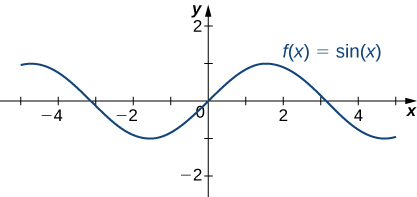
Consider the sine function \(f(x)=\sin(x)\), where \(x\) is measured in radian. The sine function is continuous everywhere,as we see in the graph above:, there fore, \(\lim_{x \rightarrow c} \sin(x)=\sin(c).\)
Thingout Loud
What is a natural domain of a function?
This leads to the following theorem.
Theorem \(\PageIndex{1}\)
If \(a\) is any number in the natural domain of the corresponding trigonometric function, then
- \(\lim_{x \rightarrow a } \sin(x)=\sin(a).\)
- \(\lim_{x \rightarrow a} \cos(x)=\cos(a).\)
- \(\lim_{x \rightarrow a} \tan(x)=\tan(a).\)
- \(\lim_{x \rightarrow a} \csc(x)=\csc(a).\)
- \(\lim_{x \rightarrow a} \sec(x)=\sec(a).\)
- \(\lim_{x \rightarrow a} \cot(x)=\cot(a).\)
- Proof
-
Since the trigonometric functions are continuous on their natural domain, the statements are valid.
Example \(\PageIndex{1}\):
Find \(\lim_{x→0} sin\left( \dfrac{x^2-1}{x-1}\right)\).
Solution:
Since \(sine\) is a continuous function and \(\lim_{x→0} \left( \dfrac{x^2-1}{x-1}\right) = \lim_{x→0} (x+1)=2\), \(\lim_{x→0} sin\left( \dfrac{x^2-1}{x-1}\right) = sin\left( \lim_{x→0}\dfrac{x^2-1}{x-1}\right) = sin ( \lim_{x→0} (x+1))=sin(2)\).
The six basic trigonometric functions are periodic and do not approach a finite limit as \(x→±∞.\) For example, \(sinx\) oscillates between \(1and−1\) (Figure). The tangent function \(x\) has an infinite number of vertical asymptotes as \(x→±∞\); therefore, it does not approach a finite limit nor does it approach \(±∞\) as \(x→±∞\) as shown in Figure.
The Squeeze Theorem
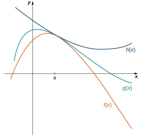
The techniques we have developed thus far work very well for algebraic functions, but we are still unable to evaluate limits of very basic trigonometric functions. The next theorem, called the squeeze theorem, proves very useful for establishing basic trigonometric limits. This theorem allows us to calculate limits by “squeezing” a function, with a limit at a point a that is unknown, between two functions having a common known limit at a. Figure illustrates this idea.
The Squeeze Theorem
Let \(f(x),g(x)\), and \(h(x)\) be defined for all x≠a over an open interval containing a. If
\[f(x)≤g(x)≤h(x)\]
for all \(x≠a\) in an open interval containing a and
\[\lim_{x→a}f(x)=L=\lim_{x→a}h(x)\]
where L is a real number, then \(\lim_{x→a}g(x)=L.\)
Example \(\PageIndex{2}\): Applying the Squeeze Theorem
Apply the squeeze theorem to evaluate \(\lim_{x→0}xcosx\).
Solution
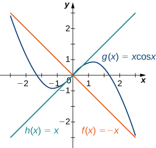
Because \(−1≤cosx≤1\) for all x, we have \(−x≤xcosx≤x\) for \(x≥0\) and \(−x≥xcosx≥x\) for \(x≤0\) (if x is negative the direction of the inequalities changes when we multiply). Since \(\lim_{x→0}(−x)=0=\lim_{x→0}x\), from the squeeze theorem, we obtain \(\lim_{x→0}xcosx=0\). The graphs of \(f(x)=−x,g(x)=xcosx\), and \(h(x)=x\) are shown in Figure.
Exercise \(\PageIndex{3}\)
Use the squeeze theorem to evaluate \(\lim_{x→0}x^2sin\frac{1}{x}\).
- Hint
-
Use the fact that \(−x^2≤x^2sin(1/x)≤x^2\) to help you find two functions such that \(x^2sin(1/x)\) is squeezed between them.
- Answer
-
0
We now use the squeeze theorem to tackle several very important limits. Although this discussion is somewhat lengthy, these limits prove invaluable for the development of the material in both the next section and the next chapter. The first of these limits is \(\lim_{θ→0}\sin θ\).
Theorem \(\PageIndex{1}\)
\[ \lim\limits_{x\to 0} \frac{\sin x}{x} = 1. \nonumber\]
- Proof
-
We begin by considering the unit circle. Each point on the unit circle has coordinates \((\cos \theta,\sin \theta)\) for some angle \(\theta\) as shown in Figure \(\PageIndex{1}\). Using similar triangles, we can extend the line from the origin through the point to the point \((1,\tan \theta)\), as shown. (Here we are assuming that \(0\leq \theta \leq \pi/2\).Later we will show that we can also consider \(\theta \leq 0\).)
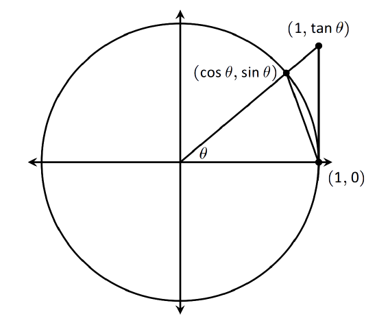
Figure \(\PageIndex{1}\): The unit circle and related triangles.Figure 1.19 shows three regions have been constructed in the first quadrant, two triangles and a sector of a circle, which are also drawn below. The area of the large triangle is \(\frac12\tan\theta\); the area of the sector is \(\theta/2\); the area of the triangle contained inside the sector is \(\frac12\sin\theta\). It is then clear from the diagram that

Multiply all terms by \(\frac{2}{\sin \theta}\), giving
\[\frac{1}{\cos\theta} \geq \frac{\theta}{\sin \theta} \geq 1.\]
Taking reciprocals reverses the inequalities, giving
\[ \cos \theta \leq \frac{\sin \theta}{\theta} \leq 1.\]
(These inequalities hold for all values of \(\theta\) near 0, even negative values, since \(\cos (-\theta) = \cos \theta\) and \(\sin (-\theta) = -\sin \theta\).)
Now take limits.
\[\lim\limits_{\theta\to 0} \cos \theta \leq \lim\limits_{\theta\to 0} \frac{\sin\theta}{\theta} \leq \lim\limits_{\theta\to 0} 1 \]
\[\cos 0 \leq \lim\limits_{\theta\to 0} \frac{\sin\theta}{\theta} \leq 1 \]
\[1 \leq \lim\limits_{\theta\to 0} \frac{\sin\theta}{\theta} \leq 1 \]
Clearly this means that \( \lim\limits_{\theta\to 0} \frac{\sin\theta}{\theta}=1\)
Example \(\PageIndex{12}\): Evaluating an Important Trigonometric Limit
Evaluate \(\lim_{θ→0}\frac{1−\cos θ}{θ}\).
Solution
In the first step, we multiply by the conjugate so that we can use a trigonometric identity to convert the cosine in the numerator to a sine:
\(\lim_{θ→0}\frac{1−\cos θ}{θ} =\lim_{θ→0}\frac{1−\cos θ}{θ}⋅\frac{1+\cos θ}{1+\cos θ}\)
=\(\lim_{θ→0}\frac{1−cos^2θ}{θ(1+\cos θ)}\)
=\(\lim_{θ→0}\frac{sin^2θ}{θ(1+\cos θ)}\)
=\(\lim_{θ→0}\frac{\sin θ}{θ}⋅\frac{\sin θ}{1+\cos θ}\)
=\(1⋅\frac{0}{2}=0\).
Therefore,
\(\lim_{θ→0}\frac{1−\cos θ}{θ}=0.\)
Exercise \(\PageIndex{10}\)
Evaluate \(\lim_{θ→0}\frac{1−\cos θ}{\sin θ}\).
- Answer
-
Multiply numerator and denominator by \(1+\cos θ\).
- Answer
-
0
Example \(\PageIndex{1}\)
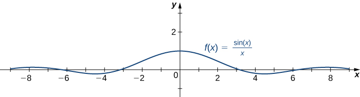
For each of the following functions \(\displaystyle f\), valuate \(\displaystyle \lim_{x\to\infty}f(x)\) and \(\displaystyle \lim_{x\to−\infty}f(x)\). Determine the horizontal asymptote(s) for \(\displaystyle f\).
- \(\displaystyle f(x)=\frac{sinx}{x}\)
- \(\displaystyle f(x)=tan^{−1}(x)\)
Solution
a. Since \(1≤sinx≤1\) for all \(x\), we have
\(\frac{−1}{x}≤\frac{sinx}{x}≤\frac{1}{x}\)
for all \(x≠0\). Also, since
\(\lim_{x→∞}\frac{−1}{x}=0=\lim_{x→∞}\frac{1}{x}\),
we can apply the squeeze theorem to conclude that
\(\lim_{x→∞}\frac{sinx}{x}=0.\)
Similarly,
\(\lim_{x→−∞}\frac{sinx}{x}=0.\)
Thus, \(f(x)=\frac{sinx}{x}\) has a horizontal asymptote of \(y=0\) and \(f(x)\) approaches this horizontal asymptote as \(x→±∞\) as shown in the following graph.
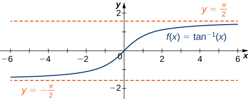
b. To evaluate \(\lim_{x→∞}tan^{−1}(x)\) and \(\lim_{x→−∞}tan^{−1}(x)\), we first consider the graph of \(y=tan(x)\) over the interval \((−π/2,π/2)\) as shown in the following graph.
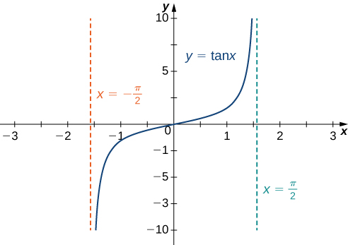
Since
\(\lim_{x→(π/2)−}tanx=∞,\)
it follows that
\(\lim_{x→∞}tan^{−1}(x)=\frac{π}{2}.\)
Similarly, since
\(\lim_{x→(π/2)^+}tanx=−∞,\)
it follows that
\(\lim_{x→−∞}tan^{−1}(x)=−\frac{π}{2}.\)
As a result, \(y=\frac{π}{2}\) and \(y=−\frac{π}{2}\) are horizontal asymptotes of \(f(x)=tan^{−1}(x)\) as shown in the following graph.
Key Concepts
- Radian measure is defined such that the angle associated with the arc of length 1 on the unit circle has radian measure 1. An angle with a degree measure of \(180\)° has a radian measure of \(\pi\) rad.
- For acute angles \(θ\),the values of the trigonometric functions are defined as ratios of two sides of a right triangle in which one of the acute angles is \(θ\).
- For a general angle \(θ\), let \((x,y)\) be a point on a circle of radius \(r\) corresponding to this angle \(θ\). The trigonometric functions can be written as ratios involving \(x\), \(y\), and \(r\).
- The trigonometric functions are periodic. The sine, cosine, secant, and cosecant functions have period \(2π\). The tangent and cotangent functions have period \(π\).
- The squzze theorem
- \(\lim_{x \to 0} \frac{\sin(x)}{x}=1\).
Source for the figure:
Diagram demonstrating trigonometric functions in the unit circle, Daniel Kleitman. RES.18-003 Calculus for Beginners and Artists. Spring 2005. Massachusetts Institute of Technology: MIT OpenCourseWare, https://ocw.mit.edu. License: Creative Commons BY-NC-SA.
Contributors and Attributions
Michael Corral (Schoolcraft College). The content of this page is distributed under the terms of the GNU Free Documentation License, Version 1.2.
Gregory Hartman (Virginia Military Institute). Contributions were made by Troy Siemers and Dimplekumar Chalishajar of VMI and Brian Heinold of Mount Saint Mary's University. This content is copyrighted by a Creative Commons Attribution - Noncommercial (BY-NC) License. http://www.apexcalculus.com/
Gilbert Strang (MIT) and Edwin “Jed” Herman (Harvey Mudd) with many contributing authors. This content by OpenStax is licensed with a CC-BY-SA-NC 4.0 license. Download for free at http://cnx.org.
Pamini Thangarajah (Mount Royal University, Calgary, Alberta, Canada)