3.4: Finite Difference Calculus

In this section, we will explore further to the method that we explained in the introduction of Quadratic sequences.

Example $\PageIndex{1}$

Create a sequence of numbers by finding a relationship between the number of points on the circumference of a circle and the number of regions created by joining the points.

Table $\PageIndex{1}$: Dividing circle

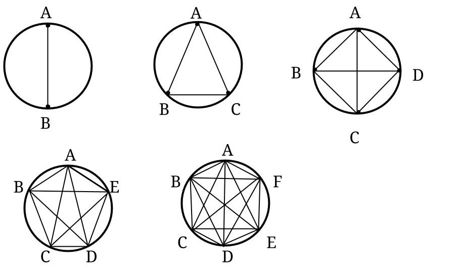
Number of points on the circle	0	1	2	3	4	5	6	7	8
Number of regions	1	1	2	4	8	16	31	57	99

Difference operator

Notation:

Let $a_n, n=0,1,2,\cdots$ be a sequence of numbers. Then the first difference is defined by $\Delta a_n = a_{n+1}-a_n, n=0,1,2,\cdots$.

The second difference is defined by $\Delta (\Delta a_n)= \Delta^2 a_n =\Delta a_{n+1}- \Delta a_n, n=0,1,2,\cdots$.

Further, $k^{th}$ difference is denoted by $\Delta^k a_n, n=k,\cdots$. We shall denote that $\Delta^0 a_n=a_n$.

Example $\PageIndex{2}$

Let $a_n=n^2$, for all $n \in \mathbb{N}$. Show that $\Delta^2 a_n=2$.

Solution

$\Delta a_n =(n+1)^2-n^2= 2n+1,$

$\Delta^2 a_n=(2(n+1)+1)-(2n+1)= 2.$

Rule

Let $k \in \mathbb{Z_+}$. Let $a_n=n^k$, for all $n \in \mathbb{N}$. Then $\Delta^k a_n=k!$.

Example $\PageIndex{3}$

Let $a_n=c^n$, for all $n \in \mathbb{N}$. Show that $\Delta a_n=(c-1) a_n$.

Solution

$\Delta a_n= c^{n+1}-c^{n}= c^n(c-1) = (c-1) a_n$.

Below are some properties of the difference operator.

Theorem $\PageIndex{1}$: Difference operator is a Linear Operator

Let $a_n$ and $b_n$ be sequences, and let $c$ be any number. Then

1. $\Delta (a_n+b_n)= \Delta a_n+ \Delta b_n$, and
2. $\Delta ( c a_n) =c \Delta a_n$.

Proof

Very simple calculation.

Definition: Falling Powers

The falling power is denoted by $x^{\underline{m}}$ and it is defined by $x (x-1)(x-2)(x-3) \cdots (x-m+1)$, with $x^{\underline{0}}=1$.

Falling powers are useful in the difference calculus because of the following property:

Theorem $\PageIndex{2}$

$\Delta n^{\underline{m}} =m \,n^{\underline{m-1}}$.

Proof

$\Delta n^{\underline{m}}= (n+1)^{\underline{m}}-n^{\underline{m}}$

$=(n+1) n (n-1)(n-2)(n-3) \cdots (n-m+2)- n (n-1)(n-2)(n-3) \cdots (n-m+1)$

$=n (n-1)(n-2)(n-3) \cdots (n-m+2) ( (n+1)-(n-m+1))$

$= n (n-1)(n-2)(n-3) \cdots (n-m+2) \,m$

$=m\, n^{\underline{m-1}}$.

Let us now consider the sequence of numbers in the example $\PageIndex{1}$.

Table $\PageIndex{2}$: Falling Powers

Number of points on the circle	0	1	2	3	4	5	6	7	8
Number of regions	1	1	2	4	8	16	31	57	99
$\Delta a_n$		0	1	2	4	8	15	26	42
$\Delta^2 a_n$			1	1	2	4	7	11	16
$\Delta^3 a_n$				0	1	2	3	4	5
$\Delta^4 a_n$					1	1	1	1	1

Since the fourth difference is constant, $a_n$ should be polynomial of degree $4$. Let's explore how to find this polynomial.

Definition

$${n \choose k } =\displaystyle \frac{ n!}{k! (n-k)!} , k \leq n, n \in \mathbb{N} \cup \{0\} .$$

Theorem $\PageIndex{2}$

$$\Delta \displaystyle {n \choose k } = \displaystyle {n \choose k-1}, k \leq n, n \in \mathbb{N} \cup \{0\} .$$

Proof

Note that $$\displaystyle {n \choose k }= \frac{1}{k!} n^{\underline{k}}.$$

Consider $\Delta {n \choose k } = \Delta ( \frac{1}{k!} n^{\underline{k}})$

$= \frac{1}{k!} \Delta( n^{\underline{k}})$

$= \frac{k}{k!} n^{\underline{(k-1)}}$

$= \frac{1}{(k-1)!} n^{\underline{(k-1)}}$

$= {n \choose k-1}$.

We can also see this by considering Pascal’s triangle.

Theorem $\PageIndex{3}$ Newton's formula

Let $a_0, a_1, a_2, \cdots$ be sequence of numbers such that $\Delta^{k+1} a_0=0.$ Then the $n$ ^th term of the original sequence is given by

$$a_n= \frac{1}{k!}(\Delta^k a_0)n^{\underline{k}} + \cdots+ a_0= a_0+ {n \choose 0 } \Delta a_1 +{n \choose 2 } \Delta^2 a_2+ \cdots + {n \choose k } \Delta^k a_k.$$

Proof

Exercise.

If $n$ ^th term of the original sequence is linear, then the first difference will be a constant. If $n$ ^th term of the original sequence is quadratic, then the second difference will be a constant. A cubic sequence has the third difference constant.

Source

• Thanks to Olivia Nannan for the diagram.
• Reference: Kunin, George B. "The finite difference calculus and applications to the interpolation of sequences." MIT Undergraduate Journal of Mathematics 232.2001 (2001): 101-9.
• Reference: Samson, D. (2006). Number patterns, cautionary tales and finite differences. Learning and Teaching Mathematics, 2006(3), 3-8.