
4.5: Measures of the Center and Variation of the Data
- Page ID
- 91563

- Recognize, describe, and calculate the measures of the center of data.
- Recognize, describe, and calculate the measures of the spread of data.
- Use Chebyshev and Empirical rules to interpret the mean and standard deviation.
Measures of the Center of the Data
The "center" of a data set is also a way of describing the location. The two most widely used measures of the "center" of the data are the mean (average) and the median. To calculate the mean weight of 50 people, add the 50 weights together and divide by 50. To find the median weight of the 50 people, order the data and find the number that splits the data into two equal parts. The median is generally a better measure of the center when there are extreme values or outliers because it is not affected by the precise numerical values of the outliers. The mean is the most common measure of the center.
The letter used to represent the sample mean is an \(x\) with a bar over it (pronounced “\(x\) bar”): \(\overline{x}\). The Greek letter \(\mu\) (pronounced "mew") represents the population mean. One of the requirements for the sample mean to be a good estimate of the population mean is for the sample taken to be truly random.
The Law of Large Numbers says that if you take samples of larger and larger sizes from any population, then the mean \(\bar{x}\) of the sample is very likely to get closer and closer to the mean of the population, \(\mu\). This is discussed in more detail later in the text.
When each value in the data set is not unique, the mean can be calculated by multiplying each distinct value by its frequency and then dividing the sum by the total number of data values. To see that both ways of calculating the mean are the same, consider the sample:
1; 1; 1; 2; 2; 3; 4; 4; 4; 4; 4
\[\bar{x} = \dfrac{1+1+1+2+2+3+4+4+4+4+4}{11} = 2.7\]
In the second calculation, the frequencies are 3, 2, 1, and 5.
You can quickly find the location of the median by using the expression
\[\dfrac{n+1}{2}\]
The letter \(n\) is the total number of data values in the sample. If \(n\) is an odd number, the median is the middle value of the ordered data (ordered smallest to largest). If \(n\) is an even number, the median is equal to the average of the two middle values after the data has been ordered. For example, if the total number of data values is 97, then
\[\dfrac{n+1}{2} = \dfrac{97+1}{2} = 49.\]
The median is the 49th value in the ordered data. If the total number of data values is 100, then
\[\dfrac{n+1}{2} = \dfrac{100+1}{2} = 50.5.\]
The median occurs midway between the 50th and 51st values. The location of the median and the value of the median are not the same. The upper case letter \(M\) is often used to represent the median. The next example illustrates the location of the median and the value of the median.
AIDS data indicating the number of months a patient with AIDS lives after taking a new antibody drug are as follows (smallest to largest):
3; 4; 8; 8; 10; 11; 12; 13; 14; 15; 15; 16; 16; 17; 17; 18; 21; 22; 22; 24; 24; 25; 26; 26; 27; 27; 29; 29; 31; 32; 33; 33; 34; 34; 35; 37; 40; 44; 44; 47
Calculate the mean and the median.
Answer
The calculation for the mean is:
\[\bar{x} = \dfrac{[3+4+(8)(2)+10+11+12+13+14+(15)(2)+(16)(2)+...+35+37+40+(44)(2)+47]}{40} = 23.6\]
To find the median, \(M\), first use the formula for the location. The location is:\[\dfrac{n+1}{2} = \dfrac{40+1}{2} = 20.5\]
Starting at the smallest value, the median is located between the 20th and 21st values (the two 24s):
3; 4; 8; 8; 10; 11; 12; 13; 14; 15; 15; 16; 16; 17; 17; 18; 21; 22; 22; 24; 24; 25; 26; 26; 27; 27; 29; 29; 31; 32; 33; 33; 34; 34; 35; 37; 40; 44; 44; 47
\[M = \dfrac{24+24}{2} = 24\]
The following data show the number of months patients typically wait on a transplant list before getting surgery. The data are ordered from smallest to largest. Calculate the mean and median.
3; 4; 5; 7; 7; 7; 7; 8; 8; 9; 9; 10; 10; 10; 10; 10; 11; 12; 12; 13; 14; 14; 15; 15; 17; 17; 18; 19; 19; 19; 21; 21; 22; 22; 23; 24; 24; 24; 24
Answer
Mean: \(3 + 4 + 5 + 7 + 7 + 7 + 7 + 8 + 8 + 9 + 9 + 10 + 10 + 10 + 10 + 10 + 11 + 12 + 12 + 13 + 14 + 14 + 15 + 15 + 17 + 17 + 18 + 19 + 19 + 19 + 21 + 21 + 22 + 22 + 23 + 24 + 24 + 24 = 544\)
\[\dfrac{544}{39} = 13.95\]
Median: Starting at the smallest value, the median is the 20th term, which is 13.
Another measure of the center is the mode. The mode is the most frequent value. There can be more than one mode in a data set as long as those values have the same frequency and that frequency is the highest.
Statistics exam scores for 20 students are as follows:
50; 53; 59; 59; 63; 63; 72; 72; 72; 72; 72; 76; 78; 81; 83; 84; 84; 84; 90; 93
Find the mode.
Answer
The most frequent score is 72, which occurs five times. Mode = 72.
The number of books checked out from the library from 25 students are as follows:
0; 0; 0; 1; 2; 3; 3; 4; 4; 5; 5; 7; 7; 7; 7; 8; 8; 8; 9; 10; 10; 11; 11; 12; 12
Find the mode.
Answer
The most frequent number of books is 7, which occurs four times. Mode = 7.
It is worth mentioning that the mean and median apply only to quantitative data, whereas the mode can be used with either quantitative or qualitative data. Thus while the mode appears to be the least useful among the three measures of central tendency, it is the only way to assess the center for qualitative data! But when working with quantitative data we still have to choose between the mean and the median. Let’s consider the following example. We have four people Ann, Beth, Connor, and Diana that make the annual salaries $30k, $50k, $50k, $70k respectfully. Their average salary is $50,000 and their median is also $50,000 dollars. Now, let’s say Elon moves in and his salary is $300,000 a year. What effect does this have on the mean and median? The new mean is $100,000 and the new median is still $50,000. Which of the two measures produces a more representative value? In this case, the median is obviously a better choice, for example if Toyota Company was considering building a Lexus or Scion dealership and they were only considering the mean it would appear that an average person in this neighborhood can afford a Lexus when in reality only one person can afford it. So what exactly the difference between the mean and the median? Unlike the mean, the median is not sensitive to the influence of a few extreme observations. Usually, we use the median for house prices and salaries and for everything else we would prefer the mean.
Suppose that in a small town of 50 people, one person earns $5,000,000 per year and the other 49 each earn $30,000. Which is the better measure of the "center": the mean or the median?
Solution
\[\bar{x} = \dfrac{5,000,000+49(30,000)}{50} = 129,400\]
\(M = 30,000\)
(There are 49 people who earn $30,000 and one person who earns $5,000,000.)
The median is a better measure of the "center" than the mean because 49 of the values are 30,000 and one is 5,000,000. The 5,000,000 is an outlier. The 30,000 gives us a better sense of the middle of the data.
In a sample of 60 households, one house is worth $2,500,000 and the rest are worth $280,000. Which is the better measure of the “center”: the mean or the median?
Answer
The median is the better measure of the “center” than the mean because 59 of the values are $280,000 and one is $2,500,000. The $2,500,000 is an outlier. The $280,000 gives us a better sense of the middle of the data.
Measures of Variation of the Data
One of the differences between the two data sets that any measure of center doesn't capture is the variety of data within the set. To describe the variation quantitatively, we use measures of variation or measures of spread. Just as there are several different measures of center, there are also several different measures of variation. In this section, we examine two of the most frequently used measures of variation: the range and standard deviation.
The range of a data set is the difference between the maximum (largest) and minimum (smallest) observations.
Find the range of the data:
| 8 | 12 | 13 | 11 | 10 | 9 | 14 | 8 | 6 | 14 | 7 | 8 | 13 |
Solution
The range of the data is the difference between the largest and the smallest values in the data set: 14−6=8
The range only measures the total variation and doesn't capture any variation between the minimum and maximum observed values. In contrast to the range, the standard deviation takes into account all the observations. It is the preferred measure of variation when the mean is used as the measure of center. Roughly speaking, the standard deviation measures variation by indicating how far, on average, the observations are from the mean. For a data set with a large amount of variation, the observations will, on average, be far from the mean; so the standard deviation will be large. For a data set with a small amount of variation, the observations will, on average, be close to the mean; so the standard deviation will be small.
If \(x\) is a number, then the difference "\(x\) – mean" is called its deviation. In a data set, there are as many deviations as there are items in the data set. The deviations are used to calculate the standard deviation. If the numbers belong to a population, in symbols a deviation is \(x - \mu\). For sample data, in symbols a deviation is \(x - \bar{x}\).
The procedure to calculate the standard deviation depends on whether the numbers are the entire population or are data from a sample. The calculations are similar, but not identical. Therefore the symbol used to represent the standard deviation depends on whether it is calculated from a population or a sample. The lower case letter s represents the sample standard deviation and the Greek letter \(\sigma\) (sigma, lower case) represents the population standard deviation. If the sample has the same characteristics as the population, then s should be a good estimate of \(\sigma\).
To calculate the standard deviation, we need to calculate the variance first. The variance is the average of the squares of the deviations (the \(x - \bar{x}\) values for a sample, or the \(x - \mu\) values for a population). The symbol \(\sigma^{2}\) represents the population variance; the population standard deviation \(\sigma\) is the square root of the population variance. The symbol \(s^{2}\) represents the sample variance; the sample standard deviation s is the square root of the sample variance. You can think of the standard deviation as a special average of the deviations.
If the numbers come from a census of the entire population and not a sample, when we calculate the average of the squared deviations to find the variance, we divide by \(N\), the number of items in the population. If the data are from a sample rather than a population, when we calculate the average of the squared deviations, we divide by n – 1, one less than the number of items in the sample.
\[s = \sqrt{\dfrac{\sum(x-\bar{x})^{2}}{n-1}} \label{eq1}\]
or
\[s = \sqrt{\dfrac{\sum f (x-\bar{x})^{2}}{n-1}} \label{eq2}\]
For the sample standard deviation, the denominator is \(n - 1\), that is one less than the sample size.
\[\sigma = \sqrt{\dfrac{\sum(x-\mu)^{2}}{N}} \label{eq3} \]
or
\[\sigma = \sqrt{\dfrac{\sum f (x-\mu)^{2}}{N}} \label{eq4}\]
For the population standard deviation, the denominator is \(N\), the number of items in the population.
In Equations \ref{eq2} and \ref{eq4}, \(f\) represents the frequency with which a value appears. For example, if a value appears once, \(f\) is one. If a value appears three times in the data set or population, \(f\) is three.
Why divide by (n-1) instead of n? Remember that the main purpose of finding a statistic is to estimate the unknown parameter. If we divide by n instead of (n-1) we will be obtaining a value which is a biased estimator for the population variance. Being biased doesn't necessarily mean bad when we know what the bias is. In this case, \sqrt{\dfrac{\sum(x-\mu)^{2}}{n}} always underestimates the true population variance by the factor of \(\frac{n}{n-1}\). After the correction, we get a desired unbiased estimator for the population variance which we call a sample variance.
In a fifth grade class, the teacher was interested in the average age and the sample standard deviation of the ages of her students. The following data are the ages for a SAMPLE of n = 20 fifth grade students. The ages are rounded to the nearest half year:
9; 9.5; 9.5; 10; 10; 10; 10; 10.5; 10.5; 10.5; 10.5; 11; 11; 11; 11; 11; 11; 11.5; 11.5; 11.5;
\[\bar{x} = \dfrac{9+9.5(2)+10(4)+10.5(4)+11(6)+11.5(3)}{20} = 10.525 \nonumber\]
The average age is 10.53 years, rounded to two places.
The variance may be calculated by using a table. Then the standard deviation is calculated by taking the square root of the variance. We will explain the parts of the table after calculating s.
| Data | Freq. | Deviations | Deviations2 | (Freq.)(Deviations2) |
|---|---|---|---|---|
| x | f | (x – \(\bar{x}\)) | (x – \(\bar{x}\))2 | (f)(x – \(\bar{x}\))2 |
| 9 | 1 | 9 – 10.525 = –1.525 | (–1.525)2 = 2.325625 | 1 × 2.325625 = 2.325625 |
| 9.5 | 2 | 9.5 – 10.525 = –1.025 | (–1.025)2 = 1.050625 | 2 × 1.050625 = 2.101250 |
| 10 | 4 | 10 – 10.525 = –0.525 | (–0.525)2 = 0.275625 | 4 × 0.275625 = 1.1025 |
| 10.5 | 4 | 10.5 – 10.525 = –0.025 | (–0.025)2 = 0.000625 | 4 × 0.000625 = 0.0025 |
| 11 | 6 | 11 – 10.525 = 0.475 | (0.475)2 = 0.225625 | 6 × 0.225625 = 1.35375 |
| 11.5 | 3 | 11.5 – 10.525 = 0.975 | (0.975)2 = 0.950625 | 3 × 0.950625 = 2.851875 |
| The total is 9.7375 |
The sample variance, \(s^{2}\), is equal to the sum of the last column (9.7375) divided by the total number of data values minus one (20 – 1):
\[s^{2} = \dfrac{9.7375}{20-1} = 0.5125 \nonumber\]
The sample standard deviation s is equal to the square root of the sample variance:
\[s = \sqrt{0.5125} = 0.715891 \nonumber\]
and this is rounded to two decimal places, \(s = 0.72\).
Note that if the 20 students were the entire population then we would use \(\mu\) instead of \(\bar{x}\), \(\sigma^{2}\) instead of \(s^{2}\), and \(\sigma\) instead of \(s\). In such a case, the population variance, \(\sigma^{2}\), is equal to the sum of the last column (9.7375) divided by the total number of data values (20):
\[\sigma^{2} = \dfrac{9.7375}{20} = 0.486875 \nonumber\]
and the population standard deviation (\sigma\) is equal to the square root of the population variance:
\[\sigma = \sqrt{0.486875} = 0.69776 \nonumber\]
In practice, USE A CALCULATOR OR COMPUTER SOFTWARE TO CALCULATE THE STANDARD DEVIATION such as this one:
Descriptive Statistics Calculator
Regardless of the tool that you use, you still need to be aware of the context and use the appropriate notation for standard deviation \(\sigma\) or \(s\).
Interpreting the Mean and Standard Deviation Together
The following lists give a few facts that provide a little more insight into what the standard deviation tells us about the distribution of the data.
For ANY data set, no matter what the distribution of the data is:
- At least 75% of the data is within two standard deviations of the mean.
- At least 89% of the data is within three standard deviations of the mean.
- At least 95% of the data is within 4.5 standard deviations of the mean.
For data having a distribution that is BELL-SHAPED and SYMMETRIC:
- Approximately 68% of the data is within one standard deviation of the mean.
- Approximately 95% of the data is within two standard deviations of the mean.
- More than 99% of the data is within three standard deviations of the mean.
The empirical rule is also known as the 68-95-99.7 rule. We will learn more about this when studying the "Normal" or "Gaussian" probability distribution in later chapters.
Suppose \(x\) is from a population with mean 50 and standard deviation 6 with bell-shape distribution.
- About 68% of the x values lie within one standard deviation of the mean. Therefore, about 68% of the x values lie between –1σ = (–1)(6) = –6 and 1σ = (1)(6) = 6 of the mean 50. The values 50 – 6 = 44 and 50 + 6 = 56 are within one standard deviation from the mean 50.
- About 95% of the x values lie within two standard deviations of the mean. Therefore, about 95% of the x values lie between –2σ = (–2)(6) = –12 and 2σ = (2)(6) = 12. The values 50 – 12 = 38 and 50 + 12 = 62 are within two standard deviations from the mean 50.
- About 99.7% of the x values lie within three standard deviations of the mean. Therefore, about 99.7% of the x values lie between –3σ = (–3)(6) = –18 and 3σ = (3)(6) = 18 from the mean 50. The values 50 – 18 = 32 and 50 + 18 = 68 are within three standard deviations of the mean 50.
The population of scores on a college entrance exam have an approximate bell-shape distribution with mean, \(\mu = 52\) points and a standard deviation, \(\sigma = 11\) points.
- About 68% of the \(y\) values lie between what two values? These values are ________________.
- About 95% of the \(y\) values lie between what two values? These values are ________________.
- About 99.7% of the \(y\) values lie between what two values? These values are ________________.
- Answer
-
a. About 68% of the values lie between the values 41 and 63.
b. About 95% of the values lie between the values 30 and 74.
c. About 99.7% of the values lie between the values 19 and 85.
It is important to note that the Empirical Rule only applies when the shape of the distribution of the data is bell-shaped and symmetric thus allowing us to sketch the following shape of the distribution based only on the two numbers: the mean and the standard deviation:
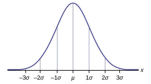
Figure \(\PageIndex{A}\)