
6.2: Continuous Random Variables


- Last updated
- Apr 18, 2022
- Save as PDF

( \newcommand{\kernel}{\mathrm{null}\,}\)
By the end of this section, the student should be able to:
- Recognize and use continuous random variables.
- Compute and interpret probabilities for a continuous random variable.
Continuous random variables have many applications. Baseball batting averages, IQ scores, the length of time a long-distance telephone call lasts, the amount of money a person carries, the length of time a computer chip lasts, and SAT scores are just a few. The field of reliability depends on a variety of continuous random variables.
The values of discrete and continuous random variables can be ambiguous. For example, if X is equal to the number of miles (to the nearest mile) you drive to work, then X is a discrete random variable. You count the miles. If X is the distance you drive to work, then you measure values of X and X is a continuous random variable. For a second example, if X is equal to the number of books in a backpack, then X is a discrete random variable. If X is the weight of a book, then X is a continuous random variable because weights are measured. How the random variable is defined is very important.

Properties of Continuous Probability Distributions
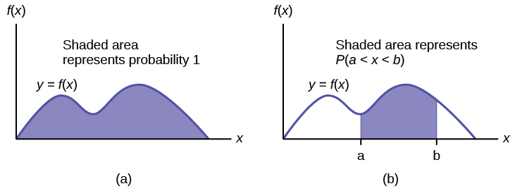
The fact that it is impossible to list all values of a continuous random variable makes it impossible to construct a probability distribution table, so instead, we are going to focus on its visual representation called a probability density function (pdf) whose graph is always on or above the horizontal axis and the total area between the graph and the horizontal axis is equal to 1. We say that a continuous random variable X is associated with a given probability density curve f(x) if the probability that X is between a and b, i.e. P(a<X<b), is equal to the area under the f(x) between a and b for any a and b.
In summary:
- The outcomes are measured, not counted.
- The entire area under the curve and above the x-axis is equal to one.
- Probability is found for intervals of x values rather than for individual x values.
- The probability that the random variable X is in the interval between the values c and d, P(c<X<d), is the area under the curve, above the x-axis, to the right of c and the left of d.
- The probability that x takes on any single individual value is zero, i.e. P(X=c)=0 for any c. The reason is that the area between the curve and the x-axis between x=c and x=c has no width, and therefore no area (area = 0). Since the probability is equal to the area, the probability is also zero.
- P(c<X<d) is the same as P(c≤X≤d) because probability is equal to area.
- The complementary rule holds i.e. P(X<c)+P(X>c)=1.
If the area to the left is 0.0228, then the area to the right is 1−0.0228=0.9772.
If the area to the left of x is 0.012, then what is the area to the right?
- Answer
-
1−0.012=0.988
The area that represents probability can be found by using geometry, formulas, technology, or probability tables. In general, calculus is needed to find the area under the curve for many probability density functions. When we use formulas to find the area in this textbook, the formulas were found by using the techniques of integral calculus. However, because most students taking this course have not studied calculus, we will not be using calculus in this textbook. There are many continuous probability distributions. When using a continuous probability distribution to model probability, the distribution used is selected to model and fit the particular situation in the best way.
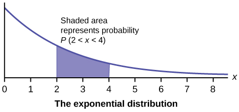
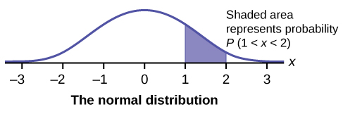
The following graphs illustrate the probability density functions and their applications for some common distributions.
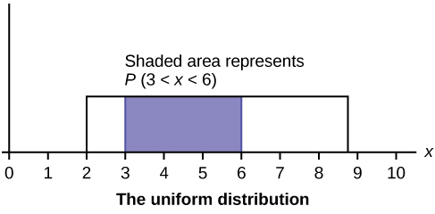
Next, we will consider one of the standard continuous random variables called uniform and some of its applications. A uniform probability density function with parameters a and b is f(x)=1b−a whose graph is a horizontal line f(x)=1b−a above the x-axis from x=a to x=b. A random variable X with such a probability density function is called a uniform random variable with parameters a and b and we denote it as X∼U(a,b). The parameters a and b are frequently called the minimum and maximum bounds.
Since the graph of a uniform probability density function is a straight horizontal line, the probability P(c<X<d) is the area of the rectangular region and thus its area can always be found using the formula:
P(c<X<d)=d−cb−a
Consider the function f(x)=120 for 0≤x≤20. The graph of f(x)=120 is a horizontal line. However, since 0≤x≤20, f(x) is restricted to the portion between x=0 and x=20, inclusive.

f(x)=120 for 0≤x≤20.
The graph of f(x)=120 is a horizontal line segment when 0≤x≤20.
The area between f(x)=120 where 0≤x≤20 and the x-axis is the area of a rectangle with base = 20 and height = 120.
AREA=20(120)=1
Suppose we want to find the area between f(x)=120 and the x-axis where 0<x<2.
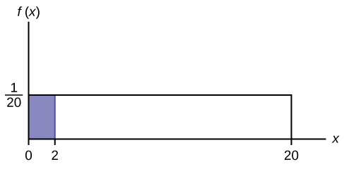
AREA=(2−0)(120)=0.1
(2−0)=2=base of a rectangle
REMINDER: area of a rectangle = (base)(height).
The area corresponds to a probability. If X has the probability density function f(x) then the probability that X is between zero and two is 0.1, which can be written mathematically as P(0<X<2)=P(X<2)=0.1.
Suppose we want to find the area between f(x)=120 and the x-axis where 4<x<15.
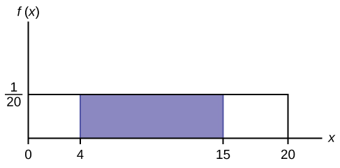
AREA=(15–4)(120)=0.55
AREA=(15–4)(120)=0.55
(15–4)=11=the base of a rectangle(15–4)=11=the base of a rectangle
The area corresponds to the probability P(4<X<15)=0.55.
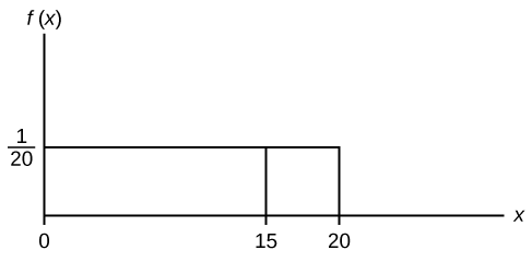
Suppose we want to find P(X=15). A vertical line x=15 has no width (or zero width). Therefore, P(X=15)=(base)(height)=(0)(120)=0
To calculate the probability that x is between two values, look at the following graph. Shade the region between x=2.3 and x=12.7. Then calculate the shaded area of a rectangle.
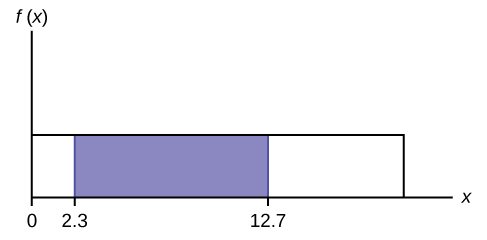
P(2.3<X<12.7)=(base)(height)=(12.7−2.3)(120)=0.52
Consider the function f(x)=18 for 0≤x≤8. Draw the graph of f(x) and find P(2.5<x<7.5).
- Answer
-
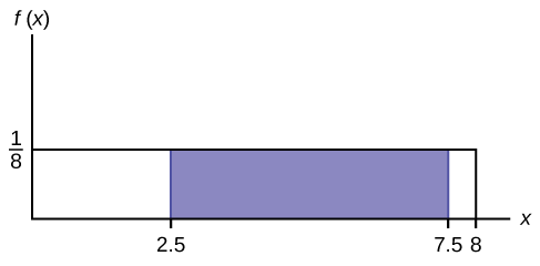
Figure 6.2.6 P(2.5<X<7.5)=0.625
Uniform random variables have many applications.
A random passenger comes to a train station through which his desired city metro train runs every 15 minutes. Find the probability that the waiting time is
(i) less than 10 minutes.
(ii) between 3 and 7 minutes.
(iii) more than 12 minutes.
Solution
The waiting time of the passenger can be estimated by a uniform random variable. Let X be the waiting time of a randomly selected passenger then it can be assumed uniform with parameters 0 and 15, i.e. X∼U(0,15). Thus:
(i) the probability that the waiting time is less than 10 minutes:
P(X<10)=width⋅height=(10−0)⋅115−0=1015=0.67
(ii) the probability that the waiting time is between 3 and 7 minutes:
P(3<X<7)=width⋅height=(7−3)⋅115−0=415=0.27
(iii) the probability that the waiting time is more than 12 minutes:
P(X>12)=width⋅height=(15−12)⋅115−0=315=0.20
A city metro train on the yellow line runs every 10 minutes during the time between 12 pm and 3 pm. Let XX be the waiting time of a randomly selected passenger between 12 pm and 3 pm. Use this information to find the probability that it takes:
i. less than 6 minutes to wait for the train?
ii. more than 7 minutes to wait for the train?
iii. between 4 and 9 minutes to wait for the train?
- Answer
-
(i) 0.6 (ii) 0.3 (iii) 0.5