
3.4: Interpreting the Mean and Standard Deviation
- Page ID
- 105823

\( \newcommand{\vecs}[1]{\overset { \scriptstyle \rightharpoonup} {\mathbf{#1}} } \)
\( \newcommand{\vecd}[1]{\overset{-\!-\!\rightharpoonup}{\vphantom{a}\smash {#1}}} \)
\( \newcommand{\dsum}{\displaystyle\sum\limits} \)
\( \newcommand{\dint}{\displaystyle\int\limits} \)
\( \newcommand{\dlim}{\displaystyle\lim\limits} \)
\( \newcommand{\id}{\mathrm{id}}\) \( \newcommand{\Span}{\mathrm{span}}\)
( \newcommand{\kernel}{\mathrm{null}\,}\) \( \newcommand{\range}{\mathrm{range}\,}\)
\( \newcommand{\RealPart}{\mathrm{Re}}\) \( \newcommand{\ImaginaryPart}{\mathrm{Im}}\)
\( \newcommand{\Argument}{\mathrm{Arg}}\) \( \newcommand{\norm}[1]{\| #1 \|}\)
\( \newcommand{\inner}[2]{\langle #1, #2 \rangle}\)
\( \newcommand{\Span}{\mathrm{span}}\)
\( \newcommand{\id}{\mathrm{id}}\)
\( \newcommand{\Span}{\mathrm{span}}\)
\( \newcommand{\kernel}{\mathrm{null}\,}\)
\( \newcommand{\range}{\mathrm{range}\,}\)
\( \newcommand{\RealPart}{\mathrm{Re}}\)
\( \newcommand{\ImaginaryPart}{\mathrm{Im}}\)
\( \newcommand{\Argument}{\mathrm{Arg}}\)
\( \newcommand{\norm}[1]{\| #1 \|}\)
\( \newcommand{\inner}[2]{\langle #1, #2 \rangle}\)
\( \newcommand{\Span}{\mathrm{span}}\) \( \newcommand{\AA}{\unicode[.8,0]{x212B}}\)
\( \newcommand{\vectorA}[1]{\vec{#1}} % arrow\)
\( \newcommand{\vectorAt}[1]{\vec{\text{#1}}} % arrow\)
\( \newcommand{\vectorB}[1]{\overset { \scriptstyle \rightharpoonup} {\mathbf{#1}} } \)
\( \newcommand{\vectorC}[1]{\textbf{#1}} \)
\( \newcommand{\vectorD}[1]{\overrightarrow{#1}} \)
\( \newcommand{\vectorDt}[1]{\overrightarrow{\text{#1}}} \)
\( \newcommand{\vectE}[1]{\overset{-\!-\!\rightharpoonup}{\vphantom{a}\smash{\mathbf {#1}}}} \)
\( \newcommand{\vecs}[1]{\overset { \scriptstyle \rightharpoonup} {\mathbf{#1}} } \)
\(\newcommand{\longvect}{\overrightarrow}\)
\( \newcommand{\vecd}[1]{\overset{-\!-\!\rightharpoonup}{\vphantom{a}\smash {#1}}} \)
\(\newcommand{\avec}{\mathbf a}\) \(\newcommand{\bvec}{\mathbf b}\) \(\newcommand{\cvec}{\mathbf c}\) \(\newcommand{\dvec}{\mathbf d}\) \(\newcommand{\dtil}{\widetilde{\mathbf d}}\) \(\newcommand{\evec}{\mathbf e}\) \(\newcommand{\fvec}{\mathbf f}\) \(\newcommand{\nvec}{\mathbf n}\) \(\newcommand{\pvec}{\mathbf p}\) \(\newcommand{\qvec}{\mathbf q}\) \(\newcommand{\svec}{\mathbf s}\) \(\newcommand{\tvec}{\mathbf t}\) \(\newcommand{\uvec}{\mathbf u}\) \(\newcommand{\vvec}{\mathbf v}\) \(\newcommand{\wvec}{\mathbf w}\) \(\newcommand{\xvec}{\mathbf x}\) \(\newcommand{\yvec}{\mathbf y}\) \(\newcommand{\zvec}{\mathbf z}\) \(\newcommand{\rvec}{\mathbf r}\) \(\newcommand{\mvec}{\mathbf m}\) \(\newcommand{\zerovec}{\mathbf 0}\) \(\newcommand{\onevec}{\mathbf 1}\) \(\newcommand{\real}{\mathbb R}\) \(\newcommand{\twovec}[2]{\left[\begin{array}{r}#1 \\ #2 \end{array}\right]}\) \(\newcommand{\ctwovec}[2]{\left[\begin{array}{c}#1 \\ #2 \end{array}\right]}\) \(\newcommand{\threevec}[3]{\left[\begin{array}{r}#1 \\ #2 \\ #3 \end{array}\right]}\) \(\newcommand{\cthreevec}[3]{\left[\begin{array}{c}#1 \\ #2 \\ #3 \end{array}\right]}\) \(\newcommand{\fourvec}[4]{\left[\begin{array}{r}#1 \\ #2 \\ #3 \\ #4 \end{array}\right]}\) \(\newcommand{\cfourvec}[4]{\left[\begin{array}{c}#1 \\ #2 \\ #3 \\ #4 \end{array}\right]}\) \(\newcommand{\fivevec}[5]{\left[\begin{array}{r}#1 \\ #2 \\ #3 \\ #4 \\ #5 \\ \end{array}\right]}\) \(\newcommand{\cfivevec}[5]{\left[\begin{array}{c}#1 \\ #2 \\ #3 \\ #4 \\ #5 \\ \end{array}\right]}\) \(\newcommand{\mattwo}[4]{\left[\begin{array}{rr}#1 \amp #2 \\ #3 \amp #4 \\ \end{array}\right]}\) \(\newcommand{\laspan}[1]{\text{Span}\{#1\}}\) \(\newcommand{\bcal}{\cal B}\) \(\newcommand{\ccal}{\cal C}\) \(\newcommand{\scal}{\cal S}\) \(\newcommand{\wcal}{\cal W}\) \(\newcommand{\ecal}{\cal E}\) \(\newcommand{\coords}[2]{\left\{#1\right\}_{#2}}\) \(\newcommand{\gray}[1]{\color{gray}{#1}}\) \(\newcommand{\lgray}[1]{\color{lightgray}{#1}}\) \(\newcommand{\rank}{\operatorname{rank}}\) \(\newcommand{\row}{\text{Row}}\) \(\newcommand{\col}{\text{Col}}\) \(\renewcommand{\row}{\text{Row}}\) \(\newcommand{\nul}{\text{Nul}}\) \(\newcommand{\var}{\text{Var}}\) \(\newcommand{\corr}{\text{corr}}\) \(\newcommand{\len}[1]{\left|#1\right|}\) \(\newcommand{\bbar}{\overline{\bvec}}\) \(\newcommand{\bhat}{\widehat{\bvec}}\) \(\newcommand{\bperp}{\bvec^\perp}\) \(\newcommand{\xhat}{\widehat{\xvec}}\) \(\newcommand{\vhat}{\widehat{\vvec}}\) \(\newcommand{\uhat}{\widehat{\uvec}}\) \(\newcommand{\what}{\widehat{\wvec}}\) \(\newcommand{\Sighat}{\widehat{\Sigma}}\) \(\newcommand{\lt}{<}\) \(\newcommand{\gt}{>}\) \(\newcommand{\amp}{&}\) \(\definecolor{fillinmathshade}{gray}{0.9}\)Section 1: Chebyshev's Rule
In this section, we will learn how get a rough idea about the data distribution from the measures of the center and variation. The idea is simple - when we have data, we want to be able to construct and communicate a visual summary, but when that is impossible, we produce the numerical summaries which are very concise and yet packed with information! Next, we will learn how to interpret the numerical summaries to communicate the shape of the distribution. For example, what do you imagine, when you hear that a dataset has the average 50 and the standard deviation 10?
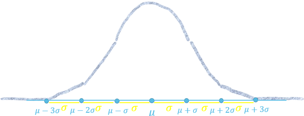
Naturally, there is a bond between the standard deviation and the mean, which can be used to unpack the information packed in these two values. Since the units of a standard deviation are the same as the units of data, it makes it easy to use it as a measuring stick on the data axis and create the scale by adding and subtracting \(1\sigma\), \(2\sigma\), and \(3\sigma\) from and to \(\mu\). We say the values are:
- within 1 standard deviation if they are between \(\mu-1\sigma\) and \(\mu+1\sigma\).
- within 2 standard deviations if they are between \(\mu-2\sigma\) and \(\mu+2\sigma\).
- within 3 standard deviations if they are between \(\mu-3\sigma\) and \(\mu+3\sigma\).
When \(\mu=50\) and \(\sigma=10\) we say the values are:
- within 1 standard deviation if they are between \(\mu-1\sigma=50-10=40\) and \(\mu+1\sigma=50+10=60\).
- within 2 standard deviations if they are between \(\mu-2\sigma=50-20=30\) and \(\mu+2\sigma=50+20=70\).
- within 3 standard deviations if they are between \(\mu-3\sigma=50-30=20\) and \(\mu+3\sigma=50+30=80\).
One other thing that we will keep an eye on while interpreting the numerical summaries is the outliers!
An outlier is an observation that appears extreme relative to the rest of the data. The rule of thumb is the three-standard-deviations rule, which states that most of the observations in any dataset lie within three standard deviations to either side of the mean, so anything beyond the three standard deviations is considered to be very unlikely and therefore satisfies the definition of an outlier.
In some books, the values that are more than two standard deviations away from the mean are called significant values that are either significantly low or significantly high, depending on whether they are below or above the mean.
When \(\mu=50\) and \(\sigma=10\) we call:
- any observation less than 20 or greater than 80 is an outlier.
- any observation less than 30 is significantly low.
- any observation more than 70 is significantly high.
It is not hard to observe that there are fewer and fewer observations the further and further away from the mean. This result was generalized by Pafnuty Chebyshev into the following theorem, named after him.
In any dataset, at least \( (1-\frac{1}{k^2})\cdot100\%\) of observations are within \(k\) standard deviations from the mean. In other words:
- At least 75% of observations are within 2 standard deviations.
- At least 89% of observations are within 3 standard deviations.
- At least 93.75% of observations are within 4 standard deviations.
When \(\mu=50\) and \(\sigma=10\) we call:
- At least 75% of observations are between 30 and 70.
- At least 89% of observations are between 20 and 80.
- At least 93.75% of observations are between 10 and 90.
The significance of the Chebyshev’s theorem is not in the exact percentages but in the fact that now we can imagine the shape of the histogram based on only two numbers.
When \(\mu=50\) and \(\sigma=10\) we expect the histogram to look somewhat like this which of course is not accurate but just a rough description of the actual histogram.

Anyway, it is better than nothing!
Consider again the president's age at inauguration:
|
42 |
43 |
46 |
47 |
47 |
47 |
48 |
49 |
49 |
|
50 |
51 |
51 |
51 |
51 |
51 |
52 |
52 |
54 |
|
54 |
54 |
54 |
54 |
55 |
55 |
55 |
55 |
56 |
|
56 |
56 |
57 |
57 |
57 |
57 |
58 |
60 |
61 |
|
61 |
61 |
62 |
64 |
64 |
65 |
68 |
69 |
70 |
In the president's age at inauguration data set, the mean is approximately 55 and the standard deviation is approximately 6.5. We can compute how much of the data exactly are within 1, 2, 3, and 4 standard deviations from the mean and confirm the Chebyshev's rule.
|
Within |
1 st. dev. = 6.5 |
2 st. dev. = 13 |
3 st. dev. = 19.5 |
4 st. dev. = 26 |
|
Between |
48.5 and 61.5 |
42 and 68 |
35.5 and 74.5 |
29 and 81 |
|
How many values? |
31/45=68.89% |
42/45=93.33% |
45/45=100% |
45/45=100% |
|
Chebyshev's Rule |
n/a |
At least 75% |
At least 89% |
At least 93.75% |
Chebyshev’s rule is always true!
So just based on the two numbers we would draw the following scale and would imaging the following shape of the distribution.

If we superimpose the actual histogram, we will be able to see that we are not that far off!

Section 2: The Empirical Rule
Previously we learned how to get a rough shape of the distribution from a given mean and standard deviation using the Chebyshev’s rule which can be applied for any dataset. Next, we will discuss the Empirical rule that allows us to better visualize the data if we can assume that it has a bell-shaped distribution.
For normal (bell-shaped) distributions the Chebyshev's estimate is too rough and can be improved.
If the distribution of the data set is or can be assumed to be approximately normal (or bell-shaped), we can apply the Empirical Rule, which states the following:
- roughly 68% of observations are within 1 standard deviation.
- roughly 95% of observations are within 2 standard deviations.
- roughly 99.7% of observations are within 3 standard deviations.
Example: When \(\mu=50\) and \(\sigma=10\):
- Roughly 68% of observations are between 40 and 60.
- Roughly 95% of observations are between 30 and 70.
- Roughly 99.7% of observations are between 20 and 80.
The significance of the Empirical Rule is that it enables us to determine the shape of the bell-curve from the mean and standard deviation only.
- Draw a horizontal axis and label the values that are 1, 2, 3, standard deviations away from the mean.
- Only 0.3% of the data are outside of 3 standard deviations – so we can draw the tails that are basically on the x-axis outside of the three standard deviations away.
- 5% of the data are outside of 2 standard deviations - continue drawing the tails towards the middle by increasing the slope by a notch.
- 32% of the data are outside of 1 standard deviation - continue drawing the tails towards the middle by increasing the slope by another notch.
- 68% of the data are within 1 standard deviation - connect the tails with the bell-shaped middle part.
According to the Empirical rule we have the following distribution of data under the curve:
- The middle 68% are evenly split into two halves – 34% each.
- The 27% of the data is between 1 and 2 standard deviations away which means 13.5% in each half.
- The 5% of the data outside of the 2 standard deviations is mainly concentrated between 2 and 3 standard deviations which means 2.5% in each tail.

We can do the same for any \(\mu\) and \(\sigma\)! For example, when \(\mu=50\) and \(\sigma=10\) we get the following:

In the president's age at inauguration data set, the mean is approximately 55 and the standard deviation is approximately 6.5. We can compute how much of the data exactly are within 1, 2, 3, and 4 standard deviations from the mean and confirm the Empirical Rule.
|
Within |
1 st. dev. = 6.5 |
2 st. dev. = 13 |
3 st. dev. = 19.5 |
4 st. dev. = 26 |
|
Between |
48.5 and 61.5 |
42 and 68 |
35.5 and 74.5 |
29 and 81 |
|
How many values? |
31/45=68.89% |
42/45=93.33% |
45/45=100% |
45/45=100% |
|
The Empirical Rule |
Approx 68% |
Approx 95% |
Approx 99.7% |
n/a |
Remember that the Empirical Rule only applies when the data distribution can be assumed normal! Assuming that the presidents’ ages are normally distributed, if we superimpose the actual histogram we will be able to see that we are not that far off!
