12.7: The Summary of Hypothesis Testing for Two Parameters

We learned altogether 6 procedures for testing statistical claims about 3 different pairs of parameters. So how do we know when and which procedure to use? Next, we will summarize all the procedures for testing hypotheses for two parameters.

First, we must determine the statistical claim that is being tested in two steps:

1. Look for the key words to identify the parameters in the claim:
   • A pair of means/averages when testing a claim about two population means.
   • A pair of proportions/percentages when testing a claim about two population proportions.
   • A pair of variances/standard deviations when testing a claim about two population variances.
2. Look for the key words that identify the inequality in the claim:
   • Less than/at most for LT
   • Not equal/different for TT
   • Greater than/at least for RT

The statistical claim in the form of an inequality is called the alternative hypothesis, and the statistical claim in the form of an equation is called the null hypothesis.

Next, we determine the procedure in the following way:

• Use the \(F\) procedure for testing claims about 2 variances.
• Use the \(Z\) procedure for testing claims about 2 proportions.
• For testing claims about two means, we first need to check whether the samples are paired or independent:
  • If they are paired, then we use One Mean \(T\) Procedure.
  • If they are independent, then we check whether the population standard deviations are known:
    • If the population standard deviations are known, then we use the \(Z\) procedure.
    • If the population standard deviations are unknown, then we check whether they can be assumed equal:
      • If unknown population standard deviations can be assumed equal, then we use the \(T\) pooled procedure.
      • If unknown population standard deviations cannot be assumed equal, then we use \(T\) non-pooled procedure. 

Remember - before applying the procedure verify all the assumptions!

So before starting the procedure we must have already figured out the significance level α which is the maximum tolerated type 1 error. The most common values for alpha are \(1\), \(5\), and \(10\%\).

Next, we compute the test statistic using a formula that is specific to each procedure. Note that we label the test statistic using the lower-case letter of the name of the involved distribution with the index zero. That is in a \(Z\)-test the test statistic is called \(z_0\), in the \(T\)-test the test statistic is called \(t_0\), and in the \(F\)-test the test statistic is called \(f_0\).

Procedure	Two Variances \(F\) Test	Two Proportions \(Z\) Test	Two Means \(Z\) Test	Two Means \(T\) Non-Pooled Test	Two Means \(T\) Pooled Test	Two Paired Means \(T\) Test
Test Statistic:	\(f_0=\frac{s^2_1}{s^2_2}\) \(df=(n_1-1, n_2-1)\)	\(z_0=\frac{\hat{p}_1-\hat{p}_2}{\sqrt{\hat{p}_p\cdot(1-\hat{p}_p)}\cdot\sqrt{\frac{1}{n_1}+\frac{1}{n_2}}}\) \(\hat{p}_p=\frac{x_1+x_2}{n_1+n_2}\)	\(z_0=\frac{\bar{x}_1-\bar{x}_2}{\sqrt{\frac{\sigma^2_1}{n_1}+\frac{\sigma^2_2}{n_2}}}\)	\(t_0=\frac{\bar{x}_1-\bar{x}_2}{\sqrt{\frac{s^2_1}{n_1}+\frac{s^2_1}{n_2}}}\)	\(t_0=\frac{\bar{x}_1-\bar{x}_2}{s_p\sqrt{\frac{1}{n_1}+\frac{1}{n_2}}}\) \(df=n_1+n_2-2\)	\(t_0=\frac{\bar{d}-\mu_0}{s_d/\sqrt{n}}\) \(df=n-1\)

To apply the formula, one must be able to understand the notation. In this step, it may be necessary to reread the question several times to extract the information.

Procedure	Two Variances \(F\) Test	Two Proportions \(Z\) Test	Two Means \(Z\) Test	Two Means \(T\) Non-Pooled Test	Two Means \(T\) Pooled Test	Two Paired Means \(T\) Test
Notation:	\(s^2_i\) sample variances	\(\hat{p}_i\) sample proportions \(\hat{p}_p\) pooled proportion \(x_i\) number of positive responses \(n_i\) sample sizes	\(\bar{x}_i\) sample means \(\sigma^2_i\) population variances \(n_i\) sample sizes	\(\bar{x}_i\) sample means \(s^2_i\) sample variances \(n_i\) sample sizes	\(\bar{x}_i\) sample means \(s^2_i\) sample variances \(s^2_p\) pooled variance \(n_i\) sample sizes	\(\bar{d}\) average difference \(\sigma^2_d\) variance of differences \(\mu_0\) mean from \(H_0\) \(n\) sample size

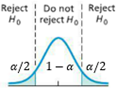
To test the claim, we can use the critical value approach. In this approach, we construct the rejection region under the probability density curve of the involved distribution based on the type of the test and the significance level alpha. The boundaries of the region are called the critical values and can be found in a similar way for all procedures. We reject the null hypothesis if the test statistic is in the rejection region.

Test Type	LT	TT	RT
RR
Critical Values	LCV: \(x_{1-\alpha}\)     RCV: DNE	LCV: \(x_{1-\alpha/2}\)     RCV: \(x_{\alpha/2}\)	LCV: DNE     RCV: \(x_\alpha\)
Reject if ...	\(x_0<x_{1-\alpha}\)	\(x_0<x_{1-\alpha/2}\) or \(x_0>x_{\alpha/2}\)	\(x_0>x_{\alpha}\)

Note that \(x_\alpha\) and \(x_0\) can be \(z_\alpha\) and \(z_0\), \(t_\alpha\) and \(t_0\), or \(\chi_\alpha^2\) and \(\chi_0^2\).

Alternatively, we can use the P-value approach. In this approach, we find the p-value depending on the test statistic and the type of the test. We reject the null hypothesis if the p-value is less than the significance level \(\alpha\).

Test Type	LT	TT	RT
P-Value
	\(P(X<x_0)\)	\(2P(X<x_0)\) or \(2P(X>x_0)\)	\(P(X>x_0)\)
Reject if ...	\(\text{P-value}<\alpha\)

Note that \(x_\alpha\) and \(x_0\) can be \(z_\alpha\) and \(z_0\), \(t_\alpha\) and \(t_0\), or \(\chi_\alpha^2\) and \(\chi_0^2\).

Due to the logic of a hypothesis testing procedure, there are only two outcomes of the procedure:

reject or not reject the null hypothesis

Note that the double negative in this case is never interpreted as a positive that is, we never-never accept the null hypothesis! Therefore, the interpretation is that we either do or do not have sufficient evidence to suggest the alternative hypothesis.

All six procedures can be summarized in the following table!

Procedure	Two Variances \(F\) Test	Two Proportions \(Z\) Test	Two Means \(Z\) Test	Two Means \(T\) Non-Pooled Test	Two Means \(T\) Pooled Test	Two Paired Means \(T\) Test
Purpose:	To test a statistical claim about two population variances	To test a statistical claim about two population proportions	To test a statistical claim about two population means
Assumptions:	Simple random sample Independent samples Normal populations	Simple random samples Independent samples \(n_i\hat{p}_i\geq10\) and \(n_i(1-\hat{p}_i\)geq10\) for \(i=1, 2\)	Simple random samples Independent samples Normal population or large samples Population standard deviations are known	Simple random samples Independent samples Normal population or large samples Population standard deviations are unknown	Simple random samples Independent samples Normal population or large samples Population standard deviations are unknown but assumed to be equal	Simple random samples Paired samples Normal population or large sample
Hypotheses:	\(H_0: \frac{\sigma^2_1}{\sigma^2_2}=k\) \(H_a: \frac{\sigma^2_1}{\sigma^2_2}?k\)	\(H_0: p_1-p_2=\Delta_0\) \(H_a: p_1-p_2?\Delta_0\)	\(H_0: \mu_1-\mu_2=\Delta_0\) \(H_a: \mu_1-\mu_2?\Delta_0\)			\(H_0: \mu_d=\mu_0\) \(H_a: \mu_d?\mu_0\)
Test Statistic:	\(f_0=\frac{s^2_1}{s^2_2}\) \(df=(n_1-1, n_2-1)\)	\(z_0=\frac{\hat{p}_1-\hat{p}_2}{\sqrt{\hat{p}_p\cdot(1-\hat{p}_p)}\cdot\sqrt{\frac{1}{n_1}+\frac{1}{n_2}}}\) \(\hat{p}_p=\frac{x_1+x_2}{n_1+n_2}\)	\(z_0=\frac{\bar{x}_1-\bar{x}_2}{\sqrt{\frac{\sigma^2_1}{n_1}+\frac{\sigma^2_2}{n_2}}}\)	\(t_0=\frac{\bar{x}_1-\bar{x}_2}{\sqrt{\frac{s^2_1}{n_1}+\frac{s^2_1}{n_2}}}\)	\(t_0=\frac{\bar{x}_1-\bar{x}_2}{s_p\sqrt{\frac{1}{n_1}+\frac{1}{n_2}}}\) \(df=n_1+n_2-2\)	\(t_0=\frac{\bar{d}-\mu_0}{s_d/\sqrt{n}}\) \(df=n-1\)
Test Type:	\(<\)		\(\neq\)		\(>\)
	LT		TT		RT
CVA: Reject if …	\(x_0<x_{1-\alpha}\)		\(x_0<x_{1-\alpha/2}\) or \(x_0>x_{\alpha/2}\)		\(x_0>x_{\alpha}\)
PVA: Reject if …	\(P(X<x_0)\)		\(2P(X<x_0)\) or \(2P(X>x_0)\)		\(P(X>x_0)\)
Interpretation:	We DO (NOT) have sufficient evidence to reject the null hypothesis in favor of the alternative hypothesis.

It is easy to see that the procedures not only have a lot in common among themselves but also with the procedures for testing the hypotheses about one parameter.