
15.1: Introduction to Regression Analysis
- Page ID
- 105881
\( \newcommand{\vecs}[1]{\overset { \scriptstyle \rightharpoonup} {\mathbf{#1}} } \)
\( \newcommand{\vecd}[1]{\overset{-\!-\!\rightharpoonup}{\vphantom{a}\smash {#1}}} \)
\( \newcommand{\id}{\mathrm{id}}\) \( \newcommand{\Span}{\mathrm{span}}\)
( \newcommand{\kernel}{\mathrm{null}\,}\) \( \newcommand{\range}{\mathrm{range}\,}\)
\( \newcommand{\RealPart}{\mathrm{Re}}\) \( \newcommand{\ImaginaryPart}{\mathrm{Im}}\)
\( \newcommand{\Argument}{\mathrm{Arg}}\) \( \newcommand{\norm}[1]{\| #1 \|}\)
\( \newcommand{\inner}[2]{\langle #1, #2 \rangle}\)
\( \newcommand{\Span}{\mathrm{span}}\)
\( \newcommand{\id}{\mathrm{id}}\)
\( \newcommand{\Span}{\mathrm{span}}\)
\( \newcommand{\kernel}{\mathrm{null}\,}\)
\( \newcommand{\range}{\mathrm{range}\,}\)
\( \newcommand{\RealPart}{\mathrm{Re}}\)
\( \newcommand{\ImaginaryPart}{\mathrm{Im}}\)
\( \newcommand{\Argument}{\mathrm{Arg}}\)
\( \newcommand{\norm}[1]{\| #1 \|}\)
\( \newcommand{\inner}[2]{\langle #1, #2 \rangle}\)
\( \newcommand{\Span}{\mathrm{span}}\) \( \newcommand{\AA}{\unicode[.8,0]{x212B}}\)
\( \newcommand{\vectorA}[1]{\vec{#1}} % arrow\)
\( \newcommand{\vectorAt}[1]{\vec{\text{#1}}} % arrow\)
\( \newcommand{\vectorB}[1]{\overset { \scriptstyle \rightharpoonup} {\mathbf{#1}} } \)
\( \newcommand{\vectorC}[1]{\textbf{#1}} \)
\( \newcommand{\vectorD}[1]{\overrightarrow{#1}} \)
\( \newcommand{\vectorDt}[1]{\overrightarrow{\text{#1}}} \)
\( \newcommand{\vectE}[1]{\overset{-\!-\!\rightharpoonup}{\vphantom{a}\smash{\mathbf {#1}}}} \)
\( \newcommand{\vecs}[1]{\overset { \scriptstyle \rightharpoonup} {\mathbf{#1}} } \)
\( \newcommand{\vecd}[1]{\overset{-\!-\!\rightharpoonup}{\vphantom{a}\smash {#1}}} \)
\(\newcommand{\avec}{\mathbf a}\) \(\newcommand{\bvec}{\mathbf b}\) \(\newcommand{\cvec}{\mathbf c}\) \(\newcommand{\dvec}{\mathbf d}\) \(\newcommand{\dtil}{\widetilde{\mathbf d}}\) \(\newcommand{\evec}{\mathbf e}\) \(\newcommand{\fvec}{\mathbf f}\) \(\newcommand{\nvec}{\mathbf n}\) \(\newcommand{\pvec}{\mathbf p}\) \(\newcommand{\qvec}{\mathbf q}\) \(\newcommand{\svec}{\mathbf s}\) \(\newcommand{\tvec}{\mathbf t}\) \(\newcommand{\uvec}{\mathbf u}\) \(\newcommand{\vvec}{\mathbf v}\) \(\newcommand{\wvec}{\mathbf w}\) \(\newcommand{\xvec}{\mathbf x}\) \(\newcommand{\yvec}{\mathbf y}\) \(\newcommand{\zvec}{\mathbf z}\) \(\newcommand{\rvec}{\mathbf r}\) \(\newcommand{\mvec}{\mathbf m}\) \(\newcommand{\zerovec}{\mathbf 0}\) \(\newcommand{\onevec}{\mathbf 1}\) \(\newcommand{\real}{\mathbb R}\) \(\newcommand{\twovec}[2]{\left[\begin{array}{r}#1 \\ #2 \end{array}\right]}\) \(\newcommand{\ctwovec}[2]{\left[\begin{array}{c}#1 \\ #2 \end{array}\right]}\) \(\newcommand{\threevec}[3]{\left[\begin{array}{r}#1 \\ #2 \\ #3 \end{array}\right]}\) \(\newcommand{\cthreevec}[3]{\left[\begin{array}{c}#1 \\ #2 \\ #3 \end{array}\right]}\) \(\newcommand{\fourvec}[4]{\left[\begin{array}{r}#1 \\ #2 \\ #3 \\ #4 \end{array}\right]}\) \(\newcommand{\cfourvec}[4]{\left[\begin{array}{c}#1 \\ #2 \\ #3 \\ #4 \end{array}\right]}\) \(\newcommand{\fivevec}[5]{\left[\begin{array}{r}#1 \\ #2 \\ #3 \\ #4 \\ #5 \\ \end{array}\right]}\) \(\newcommand{\cfivevec}[5]{\left[\begin{array}{c}#1 \\ #2 \\ #3 \\ #4 \\ #5 \\ \end{array}\right]}\) \(\newcommand{\mattwo}[4]{\left[\begin{array}{rr}#1 \amp #2 \\ #3 \amp #4 \\ \end{array}\right]}\) \(\newcommand{\laspan}[1]{\text{Span}\{#1\}}\) \(\newcommand{\bcal}{\cal B}\) \(\newcommand{\ccal}{\cal C}\) \(\newcommand{\scal}{\cal S}\) \(\newcommand{\wcal}{\cal W}\) \(\newcommand{\ecal}{\cal E}\) \(\newcommand{\coords}[2]{\left\{#1\right\}_{#2}}\) \(\newcommand{\gray}[1]{\color{gray}{#1}}\) \(\newcommand{\lgray}[1]{\color{lightgray}{#1}}\) \(\newcommand{\rank}{\operatorname{rank}}\) \(\newcommand{\row}{\text{Row}}\) \(\newcommand{\col}{\text{Col}}\) \(\renewcommand{\row}{\text{Row}}\) \(\newcommand{\nul}{\text{Nul}}\) \(\newcommand{\var}{\text{Var}}\) \(\newcommand{\corr}{\text{corr}}\) \(\newcommand{\len}[1]{\left|#1\right|}\) \(\newcommand{\bbar}{\overline{\bvec}}\) \(\newcommand{\bhat}{\widehat{\bvec}}\) \(\newcommand{\bperp}{\bvec^\perp}\) \(\newcommand{\xhat}{\widehat{\xvec}}\) \(\newcommand{\vhat}{\widehat{\vvec}}\) \(\newcommand{\uhat}{\widehat{\uvec}}\) \(\newcommand{\what}{\widehat{\wvec}}\) \(\newcommand{\Sighat}{\widehat{\Sigma}}\) \(\newcommand{\lt}{<}\) \(\newcommand{\gt}{>}\) \(\newcommand{\amp}{&}\) \(\definecolor{fillinmathshade}{gray}{0.9}\)Section 1: Fundamentals
Next, we will lay the foundation for introducing the concept of linear regression and correlation.
Let’s start with a few definitions:
A relation is any form of connection between the variables usually can be expressed as an equation.
For example, \(a+b=2\) is an equation that describes a relation between the two variables \(a\) and \(b\).
We call a variable an input variable or predictor if its value does not depend on the value of the other variable but can be chosen independently.
We call a variable an output variable or response variable if its value depends on the value of the other variable and can be computed via formula.
For example, consider the following relation:
\(V+2000t=20000\)
where \(V\) is the value ($) and \(t\) is the age of a vehicle (years).
Depending on what variable is dependent and independent, we can use one of the following equations:
\(V=-2000t+20000\) or \(t=-\frac{1}{2000}V+10\)
Now, is it the age of the vehicle that depends on the value or the value depends on the age? The answer is obvious so in the given relation the better formula for interpretation is
\(V=-2000t+20000\)
We continue with more definitions.
A relation is called linear if it can be written in the form
\(y=mx+b\)
where \(x\) is the input variable and \(y\) is the output variable.
In a linear relation, \(y=mx+b\), \(m\) is called the slope, and \(b\) is called the y-intercept.
The relation \(V=-2000t+20000\) is linear, with the slope \(m=-2000\) and the y-intercept \(b=20000\).
A graph of a linear equation is a straight line that passes through the point \((0,b)\) and rises \(|m|\) units (or drops \(|m|\) units if \(m<0\)) vertically for every horizontal change of 1 unit.
The graph of \(V=-2000t+20000\) is shown below.

An intercept is a point where the graph intersects the axis.
The graph of \(V=-2000t+20000\) has the y-intercept \(20000\) and the x-intercept \(10\).
To find the y-intercept, set the input to \(0\) and evaluate the right-hand side:
\(V=-2000\cdot0+20000\)
\(V=0+20000\)
\(V=20000\)
To find the x-intercept, set the output to \(0\) and solve the equation:
\(0=-2000\cdot t+20000\)
\(2000\cdot t=20000\)
\(t=10\)
A positive relation is a relation in which the output increases as the input increases.

A negative relation is a relation in which the output decreases as the input increases.

The relation \(V=-2000t+20000\) is a negative relation because as the age of the vehicle increases the value decreases.
In applications, the input and output variables have units, therefore everything in the equation and the graph will have units and its own interpretation:
- The y-intercept, \(b\), has the same units as the output variable and is interpreted as the output when input is zero.
- The x-intercept has the same units as the input variable and is interpreted as the input for which the output is zero.
- The slope, \(m\), has the units that are the units of the output divided by the units of the input and is interpreted as the rate of change of the output with respect to the input.
In \(V=-2000t+20000\)
- The units of the input variable \(t\) are years and the units of the output variable \(V\) are dollars.
- The y-intercept is \(b=20000\) dollars which is interpreted as the value of the vehicle when it was new (\(t=0\)).
- The x-intercept is \(t=10\) years which is interpreted as the age when the vehicle is worthless (\(V=0\)).
- The slope is \(m=-2000\) $/year which is interpreted as the rate of depreciation of the vehicle.
We can use the equation in two different ways:
- to find the output for a given input and
- to find the input with a given output.
|
Task: |
Find the output for a given input |
Find the input with a given output |
|---|---|---|
|
Given: |
\(t=5.5\) |
\(V=4000\) |
|
Solution: |
\(V=-2000\cdot5.5+20000\) \(V=-11000+20000\) \(V=9000\) |
\(4000=-2000\cdot t+20000\) \(2000\cdot t=16000\) \(t=8\) |
|
Interpretation: |
A 5.5-year-old vehicle worth $9000. |
For $4000, you can get an 8-year old vehicle. |
Imagine what you can do if such function was given for every vehicle! We CAN
- Predict the future resale value of a vehicle;
- Write-off the annual depreciation of a vehicle from taxes;
- Compare vehicles and decide which vehicle better retains its value.
However, the important question here is where does this function comes from, or in other words how does one obtain such a function or a relation?
Next, we will develop a formal procedure that will allow us to find the relation between two quantitative variables such as the value and the age of a vehicle!
Section 2: Development
So how does one reveal a relation between the two variables such as the price and the age of a car? The answer of course is in the data. To study the relation between the two variables we must collect and analyze bivariate data, in our case we must collect a sample of cars and record the age and the price of each car. We can organize such bivariate data in the form of the table:
|
Car |
Age (yr) |
Price ($100) |
|---|---|---|
|
1 |
5 |
85 |
|
2 |
4 |
103 |
|
3 |
6 |
70 |
|
4 |
5 |
82 |
|
5 |
5 |
89 |
|
6 |
5 |
98 |
|
7 |
6 |
66 |
|
8 |
6 |
95 |
|
9 |
2 |
169 |
|
10 |
7 |
70 |
|
11 |
7 |
48 |
The best way to see if there is any relation is to visualize the data! In other words, we must construct a scatterplot. When graphing the scatter plot, we decide which variable to present as independent and which as dependent. In this case, the context provides clarification – the price depends on the age of the vehicle.

Next let’s answer some questions about the data.
Q1: Does the picture suggest that there is a relation between the two variables?
A1: The image clearly shows a negative relation.
Q2: Does it look like the relation is linear?
A2: Yes. It certainly looks like a straight line can describe the relation.
Q3: What’s the graph of the linear relation?
A3: We can approximately the relation with many lines

Q4: Is there one line that is better than others?
A4: Need a criterion. The criterion that proved itself practical is the least-squares criterion.
The least-squares criterion is that the line that best fits a set of data points is one having the smallest possible sum of squared errors.
The line that describes a linear relation between any two variables is called the regression line, and its equation is called the regression equation.
So, our goal is to learn how to construct the regression line and find its equation from the data set such as in the example above.
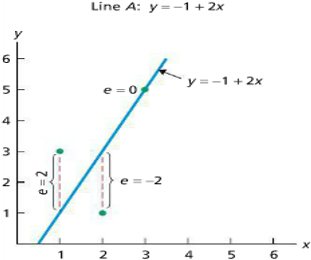
To learn the procedure, let’s consider the following small dataset along with its scatterplot:
|
|

Let’s try to fit a few lines \(y=2x-1\) and \(y=x+1\). How do we decide which of the above lines is a better fit for the data according to the least–sum of squared errors criterion? Let's compare the "fits" of two different lines by finding the sum of squared errors for each line.
For each point \((x_i,y_i )\), we find the predicted output \(\hat{y}_i\) by evaluating the regression line for each input \(x_i\); then we find the error e_i by subtracting the predicted output from the actual output observed; and then we find the squared error by squaring the error; and finally for each line we compute the sum of squared errors (\(\sum\)).
|
Line A |
Line B |
||||||||||||||||||||||||||||||||||||||||||||||||||
|---|---|---|---|---|---|---|---|---|---|---|---|---|---|---|---|---|---|---|---|---|---|---|---|---|---|---|---|---|---|---|---|---|---|---|---|---|---|---|---|---|---|---|---|---|---|---|---|---|---|---|---|
|
|

Based on this criterion we know that Line B is a better fit than Line A, but is it the best one?
Assume \(y=mx+b\) is the line of best fit then the slope and the intercept can be determined by using the following formulas:
\(m=\frac{S_{xy}}{S_{xx}}\) and \(b=\bar{y}-m\bar{x}\)
where
\(S_{xy}=\sum(x_i-\bar{x})(y_i-\bar{y})\)
\(S_{xx}=\sum(x_i-\bar{x})^2\)
\(\bar{x}=\frac{\sum x_i}{n}\)
\(\bar{y}=\frac{\sum y_i}{n}\)
The process is outlined below in the form of the table:
|
\(x\) |
\(y\) |
\(x-\bar{x}\) |
\((x-\bar{x})^2\) |
\(y-\bar{y}\) |
\((x-\bar{x})(y-\bar{y})\) |
|---|---|---|---|---|---|
|
\(1\) |
\(3\) |
\(-1\) |
\(1\) |
\(0\) |
\(0\) |
|
\(2\) |
\(1\) |
\(0\) |
\(0\) |
\(-2\) |
\(0\) |
|
\(3\) |
\(5\) |
\(1\) |
\(1\) |
\(2\) |
\(2\) |
|
\(\bar{x}=2\) |
\(\bar{y}=3\) |
\(S_{xx}=\sum=2\) |
\(S_{xy}=\sum=2\) |
\(m=\frac{S_{xy}}{S_{xx}}=\frac{2}{2}=1\)
\(b=\bar{y}-m\bar{x}=3-1\cdot2=1\)
\(y=mx+b \rightarrow y=1\cdot x+1\)
Now let's use the same process to find the line of best fit for our original data set.
|
|

The process will be summarized in the form of the table:
|
\(x\) |
\(y\) |
\(x-\bar{x}\) |
\((x-\bar{x})^2\) |
\(y-\bar{y}\) |
\((x-\bar{x})(y-\bar{y})\) |
|---|---|---|---|---|---|
|
5 |
85 |
-0.27 |
0.07 |
-3.64 |
0.99 |
|
4 |
103 |
-1.27 |
1.62 |
14.36 |
-18.28 |
|
6 |
70 |
0.73 |
0.53 |
-18.64 |
-13.55 |
|
5 |
82 |
-0.27 |
0.07 |
-6.64 |
1.81 |
|
5 |
89 |
-0.27 |
0.07 |
0.36 |
-0.10 |
|
5 |
98 |
-0.27 |
0.07 |
9.36 |
-2.55 |
|
6 |
66 |
0.73 |
0.53 |
-22.64 |
-16.46 |
|
6 |
95 |
0.73 |
0.53 |
6.36 |
4.63 |
|
2 |
169 |
-3.27 |
10.71 |
80.36 |
-263.01 |
|
7 |
70 |
1.73 |
2.98 |
-18.64 |
-32.19 |
|
7 |
48 |
1.73 |
2.98 |
-40.64 |
-70.19 |
|
\(\bar{x}=5.27\) |
\(\bar{y}=8.64\) |
\(S_{xx}=20.18\) |
\(S_{xy}=-408.91\) |
||
\(m=\frac{S_{xy}}{S_{xx}}=\frac{-408.91}{20.18}=-20.26\)
\(b=\bar{y}-m\bar{x}=88.636-(-20.26)\cdot5.273=195.47\)
\(y=mx+b \rightarrow y=-20.26\cdot x+195.47\)
\(V=-20.26t+195.47\)
|
Units |
Interpretation |
|
|---|---|---|
|
\(m=-20.26\) |
$100/year |
depreciation rate is $2026/year |
|
\(b=195.47\) |
$100 |
the price of a new car is $19547 |
We can use the equation in two different ways – to find the output for a given input and to find the input with a given output.
|
Task: |
Find the output for a given input |
Find the input with a given output |
|---|---|---|
|
Given: |
\(t=5.5\) |
\(V=40.00\) |
|
Solution: |
\(V=-20.26\cdot5.5+195.47\) \(V=-111.43+195.47\) \(V=84.04\) |
\(40.00=-20.26\cdot t+195.47\) \(20.26\cdot t=195.47\) \(t=7.7\) |
|
Interpretation: |
A 5.5-year-old vehicle worth $8404. |
For $4000, you can get a 7.7-year old vehicle. |
A few more definitions.
An extrapolation is trying to use the regression line outside of the domain which may lead to inaccurate results.
So technically, in our case the x and y intercepts are examples of extrapolation. Extrapolation may or may not make sense and it depends on the context.
An influential observation is an observation whose removal causes the regression equation to change considerably.
In our example the point \((2, 169)\) is such an observation because if it is removed the equation of the regression line changes significantly.
An outlier is an observation that lies too far from the regression line, relative to other data points.
It is important to distinguish between influential observations and outliers!
Section 3: Correlation
Now that we know how to find a regression line, we want to answer some interesting questions.
It appears that the formula can be applied to any data set, and it is true - here are the examples of the regression lines superimposed on various data sets.

As you can see all three data sets have the same linear regression, however there are some clear distinctions between the data sets. Here is another example of such behavior.

This means that some data sets have "stronger"/"more obvious" linear relations than others.
To determine how strong the linear relation between the variables we introduce the coefficient of determination, \(r^2\). To compute the coefficient of determination, we have the formula:
\(r^2=\frac{S_{xy}^2}{S_{xx}S_{yy}}\)
Find the coefficient of determination of the line of best fit for the following dataset:
|
\(x\) |
\(y\) |
|---|---|
|
1 |
3 |
|
2 |
1 |
|
3 |
5 |
Solution
To find the coefficient of determination of the line of best fit we set up the following table:
|
\(x\) |
\(y\) |
\(x-\bar{x}\) |
\((x-\bar{x})^2\) |
\(y-\bar{y}\) |
\((y-\bar{y})^2\) |
\((x-\bar{x})(y-\bar{y})\) |
|---|---|---|---|---|---|---|
|
1 |
3 |
-1 |
1 |
0 |
0 |
0 |
|
2 |
1 |
0 |
0 |
-2 |
4 |
0 |
|
3 |
5 |
1 |
1 |
2 |
4 |
2 |
|
\(\bar{x}=2\) |
\(\bar{y}=3\) |
\(S_{xx}=\sum=2\) |
\(S_{yy}=\sum=8\) |
\(S_{xy}=\sum=2\) |
\(r^2=\frac{S_{xy}^2}{S_{xx}S_{yy}}=\frac{2^2}{2\cdot8}=0.25\)
The coefficient of determination is a measure of how strong is the linear relation between the variables: \(r=1\) corresponds to a perfect linear relation, and \(r=0\) corresponds to the absence of any linear relation. In our example above, \(r^2=0.25\) which is an indicator that linear relation between the variables for which the data were presented is not strong.
Can you guess which scatterplots below have the highest \(r^2\)? How about the lowest?


The charts on the left demonstrate a perfect linear relation so the coefficient of determination is equal to 1. The charts in the center and on the right demonstrate a less than perfect linear relation so the coefficient of determination is much less than 1.
While the scatterplots on the left have the same \(r^2=1\) there is a clear difference between them. To quantify this difference, we use the linear correlation coefficient, \(r\).
To compute the linear correlation coefficient, we have the formula:
\(r=\frac{\frac{1}{n-1}S_{xy}}{S_x S_y}\)
Find the coefficient of determination of the line of best fit for the following dataset:
|
\(x\) |
\(y\) |
|---|---|
|
1 |
3 |
|
2 |
1 |
|
3 |
5 |
Solution
To find the linear correlation coefficient of the line of best fit we set up the following table:
|
\(x\) |
\(y\) |
\(x-\bar{x}\) |
\((x-\bar{x})^2\) |
\(y-\bar{y}\) |
\((y-\bar{y})^2\) |
\((x-\bar{x})(y-\bar{y})\) |
|---|---|---|---|---|---|---|
|
1 |
3 |
-1 |
1 |
0 |
0 |
0 |
|
2 |
1 |
0 |
0 |
-2 |
4 |
0 |
|
3 |
5 |
1 |
1 |
2 |
4 |
2 |
|
\(\bar{x}=2\) |
\(\bar{y}=3\) |
\(s_x=\sqrt{S_{xx}/(n-1)}=1\) |
\(s_y=\sqrt{S_{yy}/(n-1)}=2\) |
\(S_{xy}=\sum=2\) |
||
\(r=\frac{\frac{1}{n-1}S_{xy}}{S_x S_y}=\frac{\frac{1}{3-1}\cdot2}{1\cdot2}=0.5\)
The linear correlation coefficient is another measure of how strong is the linear relation between the variables: \(r=+1\) corresponds to a perfect positive linear relation, and \(r=-1\) corresponds to a perfect negative linear relation. And the reason why it is denoted by \(r\) is because of the relation between the linear correlation coefficient and coefficient of determination:
\((r)^2=r^2\)
In our example above, \(r=0.5\) which is an indicator that we have a positive linear relation between the variables for which the data were presented.
We finished the development of the procedure that allows us to find and interpret the linear regression line along with the coefficient of determination and the linear correlation coefficient.