Solving right triangles for angles
In Section 5.5, we used trigonometry on a right triangle to solve for the sides of a triangle given one side and an additional angle. Using the inverse trig functions, we can solve for the angles of a right triangle given two sides.
Example \(\PageIndex{1}\)
An airplane needs to fly to an airfield located 300 miles east and 200 miles north of its current location. At what heading should the airplane fly? In other words, if we ignore air resistance or wind speed, how many degrees north of east should the airplane fly?
Solution
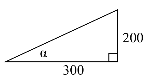
We might begin by drawing a picture and labeling all of the known information.

Drawing a triangle, we see we are looking for the angle \(\alpha\). In this triangle, the side opposite the angle \(\alpha\) is 200 miles and the side adjacent is 300 miles. Since we know the values for the opposite and adjacent sides, it makes sense to use the tangent function.
\[\tan (\alpha )=\dfrac{200}{300} \nonumber\]
Using the inverse,
\[\alpha =\tan ^{-1} \left(\dfrac{200}{300} \right)\approx 0.588 \nonumber\]
or equivalently about 33.7 degrees.
The airplane needs to fly at a heading of 33.7 degrees north of east.
Example \(\PageIndex{2}\)
OSHA safety regulations require that the base of a ladder be placed 1 foot from the wall for every 4 feet of ladder length (http://www.osha.gov/SLTC/etools/cons.../4ladders.html). Find the angle such a ladder forms with the ground.
Solution
For any length of ladder, the base needs to be one quarter of the distance the foot of the ladder is away from the wall. Equivalently, if the base is \(a\) feet from the wall, the ladder can be \(4a\) feet long. Since \(a\) is the side adjacent to the angle and \(4a\) is the hypotenuse, we use the cosine function.a
\[\cos (\theta )=\dfrac{a}{4a} =\dfrac{1}{4} \nonumber\]
Using the inverse
\[\theta =\cos ^{-1} \left(\dfrac{1}{4} \right)\approx 75.52\, \text{degrees}\nonumber\]
The ladder forms a 75.52 degree angle with the ground.
Exercise \(\PageIndex{1}\)
A cable that anchors the center of the London Eye Ferris wheel to the ground must be replaced. The center of the Ferris wheel is 70 meters above the ground and the second anchor on the ground is 23 meters from the base of the wheel. What is the angle from the ground up to the center of the Ferris wheel and how long is the cable?
- Answer
-
Angle of elevation for the cable is 71.81 degrees and the cable is 73.68 m long
Example \(\PageIndex{3}\)
In a video game design, a map shows the location of other characters relative to the player, who is situated at the origin, and the direction they are facing. A character currently shows on the map at coordinates (-3, 5). If the player rotates counterclockwise by 20 degrees, then the objects in the map will correspondingly rotate 20 degrees clockwise. Find the new coordinates of the character.
Solution
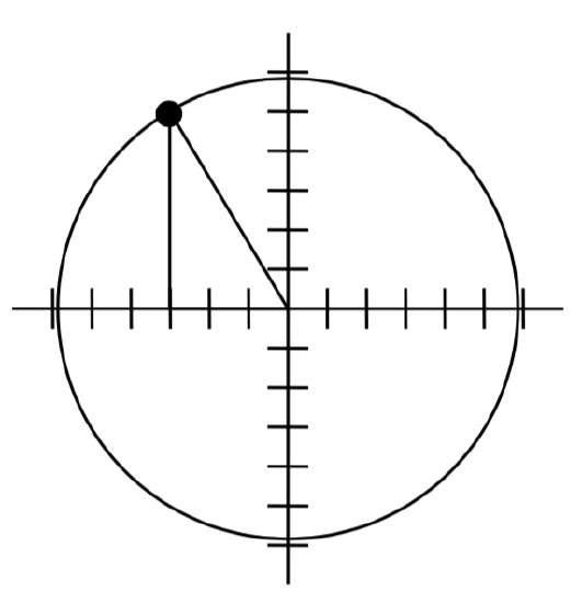
To rotate the position of the character, we can imagine it as a point on a circle, and we will change the angle of the point by 20 degrees. To do so, we first need to find the radius of this circle and the original angle.

Drawing a right triangle inside the circle, we can find the radius using the Pythagorean Theorem:
\[\begin{array}{l} {\left(-3\right)^{2} +5^{2} =r^{2} } \\ {r=\sqrt{9+25} =\sqrt{34} } \end{array}\nonumber\]
To find the angle, we need to decide first if we are going to find the acute angle of the triangle, the reference angle, or if we are going to find the angle measured in standard position. While either approach will work, in this case we will do the latter. Since for any point on a circle we know\(x=r\cos (\theta )\), using our given information we get
\[ \begin{align*} -3&=\sqrt{34} \cos (\theta ) \\[4pt] \dfrac{-3}{\sqrt{34} } &=\cos (\theta ) \\[4pt] \theta &=\cos ^{-1} \left(\dfrac{-3}{\sqrt{34} } \right)\approx 120.964{}^\circ \end{align*}\]
While there are two angles that have this cosine value, the angle of 120.964 degrees is in the second quadrant as desired, so it is the angle we were looking for.
Rotating the point clockwise by 20 degrees, the angle of the point will decrease to 100.964 degrees. We can then evaluate the coordinates of the rotated point
\[\begin{align*} x &= \sqrt{34} \text{cos} (100.964^{\circ}) \approx -1.109 \\[4pt] y &= \sqrt{34} \text{sin} (100.964^{\circ}) \approx 5.725 \end{align*}\]
The coordinates of the character on the rotated map will be (-1.109, 5.725).
Modeling with sinusoidal functions
Many modeling situations involve functions that are periodic. Previously we learned that sinusoidal functions are a special type of periodic function. Problems that involve quantities that oscillate can often be modeled by a sine or cosine function and once we create a suitable model for the problem we can use that model to answer various questions.
Example \(\PageIndex{4}\)
The hours of daylight in Seattle oscillate from a low of 8.5 hours in January to a high of 16 hours in July (www.mountaineers.org/seattle/...ylightHrs.html). When should you plant a garden if you want to do it during a month where there are 14 hours of daylight?
Solution
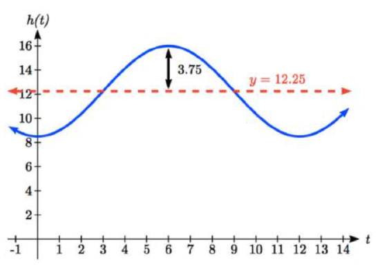
To model this, we first note that the hours of daylight oscillate with a period of 12 months. \(B=\dfrac{2\pi }{12} =\dfrac{\pi }{6}\) corresponds to the horizontal stretch, found by using the ratio of the original period to the new period.

With a low of 8.5 and a high of 16, the midline will be halfway between these values, at
\[\dfrac{16+8.5}{2} =12.25.\nonumber\]
The amplitude will be half the difference between the highest and lowest values:
\[\dfrac{16-8.5}{2} =3.75\nonumber\]
or equivalently the distance from the midline to the high or low value, 16-12.25=3.75.
Letting January be \(t = 0\), the graph starts at the lowest value, so it can be modeled as a flipped cosine graph. Putting this together, we get a model:
\[h(t)=-3.75\cos \left(\dfrac{\pi }{6} t\right)+12.25\nonumber\]
\(h(t)\) is our model for hours of day light t months after January.
To find when there will be 14 hours of daylight, we solve \(h(t) = 14\).
\[14=-3.75\cos \left(\dfrac{\pi }{6} t\right)+12.25\nonumber\]Isolating the cosine
\[1.75=-3.75\cos \left(\dfrac{\pi }{6} t\right)\nonumber\]Subtracting 12.25 and dividing by -3.75
\[-\dfrac{1.75}{3.75} =\cos \left(\dfrac{\pi }{6} t\right)\nonumber\]Using the inverse
\[\dfrac{\pi }{6} t=\cos ^{-1} \left(-\dfrac{1.75}{3.75} \right)\approx 2.0563\nonumber\]multiplying by the reciprocal
\[t=2.0563\cdot \dfrac{6}{\pi } =3.927\nonumber\]
\(t=3.927\) months past January
There will be 14 hours of daylight 3.927 months into the year, or near the end of April.
While there would be a second time in the year when there are 14 hours of daylight, since we are planting a garden, we would want to know the first solution, in spring, so we do not need to find the second solution in this case.
Exercise \(\PageIndex{2}\)
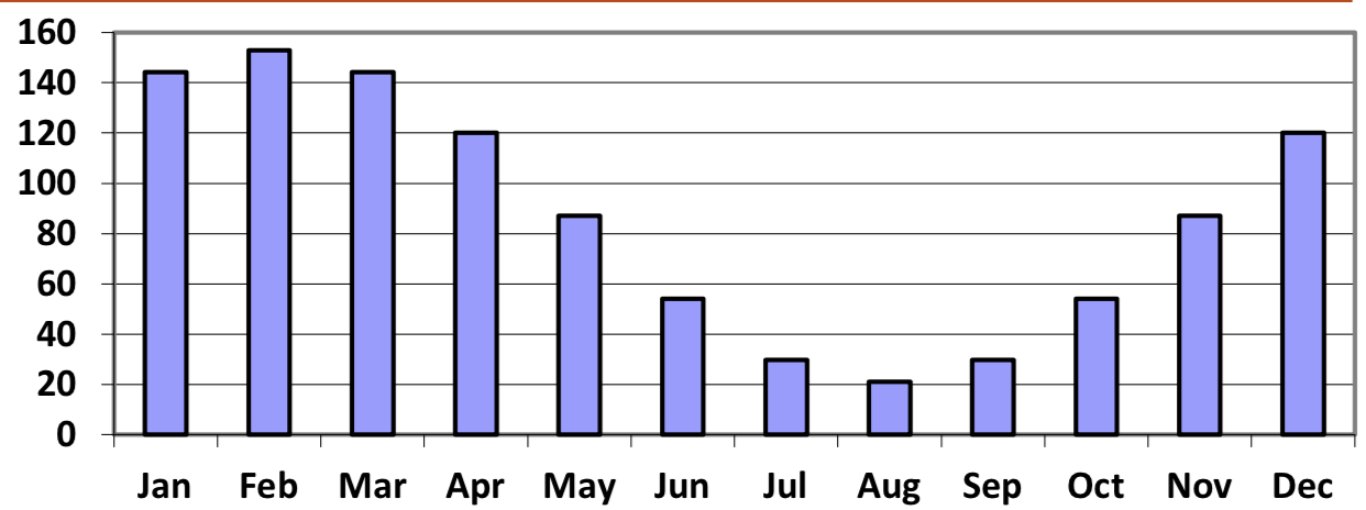
The author’s monthly gas usage (in therms) is shown here. Find a function to model the data.

- Answer
-
Approximately \[G(t)=66\cos \left(\dfrac{\pi }{6} (t-1)\right)+87\nonumber\]
Example \(\PageIndex{6}\)
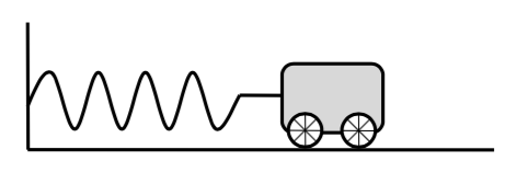
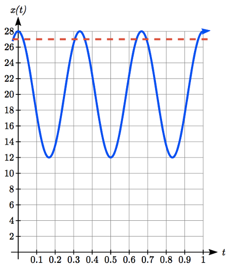
An object is connected to the wall with a spring that has a natural length of 20 cm. The object is pulled back 8 cm past the natural length and released. The object oscillates 3 times per second. Find an equation for the horizontal position of the object ignoring the effects of friction. How much time during each cycle is the object more than 27 cm from the wall?

Solution
If we use the distance from the wall, \(x\), as the desired output, then the object will oscillate equally on either side of the spring’s natural length of 20, putting the midline of the function at 20 cm.
If we release the object 8 cm past the natural length, the amplitude of the oscillation will be 8 cm.
We are beginning at the largest value and so this function can most easily be modeled using a cosine function.
Since the object oscillates 3 times per second, it has a frequency of 3 and the period of one oscillation is 1/3 of second. Using this we find the horizontal compression using the ratios of the periods: \(\dfrac{2\pi }{1/3} =6\pi\).
Using all this, we can build our model:
\[x(t)=8\cos \left(6\pi {\kern 1pt} t\right)+20 \nonumber\]
To find when the object is 27 cm from the wall, we can solve \(x(t) = 27\)
\[27=8\cos \left(6\pi {\kern 1pt} t\right)+20\nonumber\]Isolating the cosine
\[7=8\cos \left(6\pi {\kern 1pt} t\right)\nonumber\]
\[\dfrac{7}{8} =\cos \left(6\pi {\kern 1pt} t\right)\nonumber\]Using the inverse
\[6\pi {\kern 1pt} t=\cos ^{-1} \left(\dfrac{7}{8} \right)\approx 0.505\nonumber\]
\[t=\dfrac{0.505}{6\pi } =0.0268\nonumber\]

Based on the shape of the graph, we can conclude that the object will spend the first 0.0268 seconds more than 27 cm from the wall. Based on the symmetry of the function, the object will spend another 0.0268 seconds more than 27 cm from the wall at the end of the cycle. Altogether, the object spends 0.0536 seconds each cycle at a distance greater than 27 cm from the wall.
In some problems, we can use trigonometric functions to model behaviors more complicated than the basic sinusoidal function.
Example \(\PageIndex{7}\)
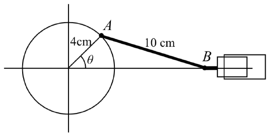
A rigid rod with length 10 cm is attached to a circle of radius 4 cm at point \(A\) as shown here. The point \(B\) is able to freely move along the horizontal axis, driving a piston (For an animation of this situation, see www.mathdemos.org/mathdemos/s...pp/engine1.gif). If the wheel rotates counterclockwise at 5 revolutions per second, find the location of point \(B\) as a function of time. When will the point \(B\) be 12 cm from the center of the circle?

Solution
To find the position of point \(B\), we can begin by finding the coordinates of point \(A\). Since it is a point on a circle with radius 4, we can express its coordinates as \((4\cos (\theta ),4\sin (\theta ))\), where \(\theta\) is the angle shown.
The angular velocity is 5 revolutions per second, or equivalently 10\(\pi \) radians per second. After \(t\) seconds, the wheel will rotate by \(\theta =10\pi {\kern 1pt} t\) radians. Substituting this, we can find the coordinates of \(A\) in terms of \(t\).
\[(4\cos (10\pi {\kern 1pt} t),4\sin (10\pi {\kern 1pt} t))\nonumber\]
Notice that this is the same value we would have obtained by observing that the period of the rotation is 1/5 of a second and calculating the stretch/compression factor:
\[\dfrac{"original"}{"new"}\dfrac{2\pi}{1/5} = 10 \pi\nonumber\]
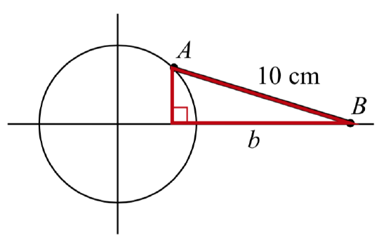
Now that we have the coordinates of the point \(A\), we can relate this to the point \(B\). By drawing a vertical line segment from \(A\) to the horizontal axis, we can form a right triangle. The height of the triangle is the \(y\) coordinate of the point \(A\): \[4\sin (10\pi {\kern 1pt} t)\nonumber\]
Using the Pythagorean Theorem, we can find the base length of the triangle:
\[\left(4\sin (10\pi {\kern 1pt} t)\right)^{2} +b^{2} =10^{2}\nonumber\]
\[b^{2} =100-16\sin ^{2} (10\pi {\kern 1pt} t)\nonumber\]
\[b=\sqrt{100-16\sin ^{2} (10\pi {\kern 1pt} t)}\nonumber\]
Looking at the \(x\) coordinate of the point \(A\), we can see that the triangle we drew is shifted to the right of the \(y\) axis by \(4\cos (10\pi {\kern 1pt} t)\). Combining this offset with the length of the base of the triangle gives the \(x\) coordinate of the point \(B\):
\[x(t)=4\cos (10\pi {\kern 1pt} t)+\sqrt{100-16\sin ^{2} (10\pi {\kern 1pt} t)}\nonumber\]
To solve for when the point B will be 12 cm from the center of the circle, we need to solve \(x(t) = 12\).
\[12=4\cos (10\pi {\kern 1pt} t)+\sqrt{100-16\sin ^{2} (10\pi {\kern 1pt} t)}\nonumber\]Isolate the square root
\[12-4\cos (10\pi {\kern 1pt} t)=\sqrt{100-16\sin ^{2} (10\pi {\kern 1pt} t)}\nonumber\]Square both sides
\[\left(12-4\cos (10\pi {\kern 1pt} t)\right)^{2} =100-16\sin ^{2} (10\pi {\kern 1pt} t)\nonumber\]Expand the left side
\[144-96\cos (10\pi {\kern 1pt} t)+16\cos ^{2} (10\pi {\kern 1pt} t)=100-16\sin ^{2} (10\pi {\kern 1pt} t)\nonumber\]Move all terms to the left
\[44-96\cos (10\pi {\kern 1pt} t)+16\cos ^{2} (10\pi {\kern 1pt} t)+16\sin ^{2} (10\pi {\kern 1pt} t)=0\nonumber\]Factor out 16
\[44-96\cos (10\pi {\kern 1pt} t)+16\left(\cos ^{2} (10\pi {\kern 1pt} t)+\sin ^{2} (10\pi {\kern 1pt} t)\right)=0\nonumber\]
At this point, we can utilize the Pythagorean Identity, which tells us that
\[\cos ^{2} (10\pi {\kern 1pt} t)+\sin ^{2} (10\pi {\kern 1pt} t)=1\nonumber\]
Using this identity, our equation simplifies to
\[44-96\cos (10\pi {\kern 1pt} t)+16=0\nonumber\]Combine the constants and move to the right side
\[-96\cos (10\pi {\kern 1pt} t)=-60\nonumber\]Divide
\[\cos (10\pi {\kern 1pt} t)=\dfrac{60}{96}\nonumber\]Make a substitution
\[\cos (u)=\dfrac{60}{96}\nonumber\]
\[u=\cos ^{-1} \left(\dfrac{60}{96} \right)\approx 0.896\nonumber\]By symmetry we can find a second solution
\[u=2\pi -0.896=5.388\nonumber\]Undoing the substitution
\[10\pi {\kern 1pt} t=0.896\text{, so }t = 0.0285\nonumber\]
\[10\pi {\kern 1pt} t=5.388\text{, so }t = 0.1715\nonumber\]
The point \(B\) will be 12 cm from the center of the circle 0.0285 seconds after the process begins, 0.1715 seconds after the process begins, and every 1/5 of a second after each of those values.


